Machine Learning for Flow Cytometry#
One of the directions cytoflow is going in that I’m most excited
about is the application of advanced machine learning methods to flow
cytometry analysis. After all, cytometry data is just a high-dimensional
data set with many data points: making sense of it can take advantage of
some of the sophisticated methods that have seen great success with
other high-throughput biological data (such as microarrays.)
The following notebook demonstrates a heavily-commented machine learning
method, Gaussian Mixture Models, applied to the demo data set we worked
with in “Basic Cytometry.” Then, there are briefer examples of some of
the other machine learning methods that are implemented in cytoflow.
Import cytoflow.
import cytoflow as flow

# if your figures are too big or too small, you can scale them by changing matplotlib's DPI
import matplotlib
matplotlib.rc('figure', dpi = 160)
We have two Tubes of data that we specify were treated with two
different concentrations of the inducer Doxycycline.
tube1 = flow.Tube(file = 'data/RFP_Well_A3.fcs',
                  conditions = {"Dox" : 10.0})
tube2 = flow.Tube(file='data/CFP_Well_A4.fcs',
                  conditions = {"Dox" : 1.0})

import_op = flow.ImportOp(conditions = {"Dox" : "float"},
                          tubes = [tube1, tube2],
                          channels = {'V2-A' : 'V2-A',
                                      'Y2-A' : 'Y2-A'})

ex = import_op.apply()
Let’s look at the histogram of the Y2-A channel (on a logicle
plot scale).
flow.HistogramView(scale = 'logicle',
                   channel = 'Y2-A').plot(ex)
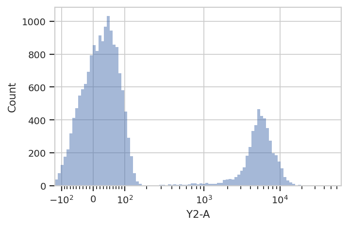
This data looks bimodal to me! Not perfect Gaussians, but close enough that using a Gaussian Mixture Model will probably let us separate them.
Let’s use the GaussianMixtureOp to separate these two populations.
In operations that are paramterized by data (either an Experiment or
some auxilliary FCS file), cytoflow separates the estimation of
module parameters from their application. Thus, after instantiating the
operation, you call estimate() to estimate the model parameters.
Those parameters stay associated with the operation instance in the same
way instances of ThresholdOp have the gate threshold as an instance
attribute.
Additionally, many modules, including GaussianMixtureModelOp, have a
default_view() factory method that returns a diagnostic plot so you
can check to see that the parameter estimation worked. This is
particularly important for unsupervised learning methods! In this case,
the GaussianMixtureModelOp’s default_view() returns a View
that plots a histogram, colored by the component each event was assigned
to, and an overlay of the Gaussian distributions on top of the
histogram.
g = flow.GaussianMixtureOp(name = "Gauss",
                           channels = ["Y2-A"],
                           scale = {"Y2-A" : "logicle"},
                           num_components = 2)

g.estimate(ex)
g.default_view().plot(ex)
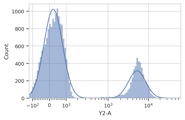
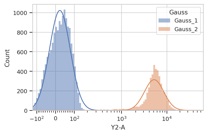
Excellent. It looks like the GMM found the two distributions we were
looking for. Let’s call apply(), then use the operation’s default
view to plot the new Experiment.
ex2 = g.apply(ex)
g.default_view().plot(ex2)
/home/brian/src/cytoflow/cytoflow/operations/base_op_views.py:376: CytoflowViewWarning: Setting 'huefacet' to 'Gauss'
apply() the GaussianMixtureModelOp, it adds a new
piece of metadata to each event in the data set: a condition whose
name that’s the same as the name of the operation (in this case,
Gauss).{Name}_{#}, where {Name} is the name of the
operation and {#} is which population had theGauss_1 or Gauss_2.ex2.data.head()
| Dox | V2-A | Y2-A | Gauss | |
|---|---|---|---|---|
| 0 | 10.0 | 41.593452 | 109.946274 | Gauss_1 |
| 1 | 10.0 | 103.437637 | 5554.108398 | Gauss_2 |
| 2 | 10.0 | -271.375580 | 81.835281 | Gauss_1 |
| 3 | 10.0 | -26.212378 | -54.120304 | Gauss_1 |
| 4 | 10.0 | 44.559933 | -10.542595 | Gauss_1 |
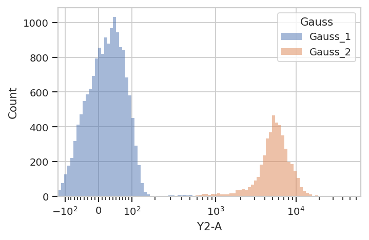
We can use that new condition to plot or compute or otherwise operate on each of the populations separately:
flow.HistogramView(channel = "Y2-A",
                   scale = "logicle",
                   huefacet = "Gauss").plot(ex2)
There’s an important subtlety to notice here. In the plot above, we set
the data scale on the HistogramView, but prior to that we passed
scale = {"Y2-A" : "logicle"} to the GaussianMixtureOp
operation. We did so in order to fit the gaussian model to the scaled
data, as opposed to the raw data.
This is an example of a broader design goal: unlike many quantitative
cytometry pipelines, cytoflow does not re-scale the underlying data;
rather, it transforms it before displaying it. Frequently it is useful
to perform the same transformation before doing data-driven things, so
many modules that have an estimate() function also allow you to
specify a scale.
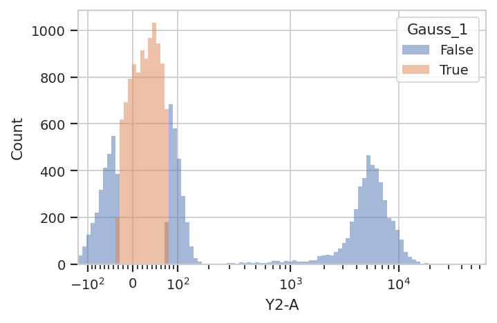
A 1-dimensional gaussian mixture model works well if the populations are
well-separated. However, if they’re closer together, you may only want
to keep events that are “clearly” in one distribution or another. One
way to accomplish this by passing a sigma parameter to
GaussianMixtureOp. This doesn’t change the behavior of
estimate(), but when you apply() the operation it creates new
conditions, one for each population. The conditions are named
{Name}_{#}, where {Name} is the name of the operation and
{#} is the index of the population. The value of the condition is
True for an event if that event is within sigma standard
deviations of the population mean.
g = flow.GaussianMixtureOp(name = "Gauss",
channels = ["Y2-A"],
scale = {"Y2-A" : "logicle"},
num_components = 2,
sigma = 1)
g.estimate(ex)
ex2 = g.apply(ex)
flow.HistogramView(channel = "Y2-A",
huefacet = "Gauss_1",
scale = "logicle").plot(ex2)
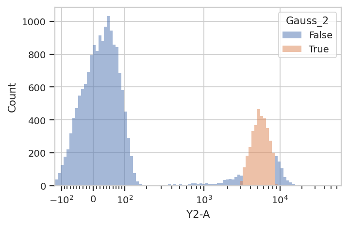
flow.HistogramView(channel = "Y2-A",
huefacet = "Gauss_2",
scale = "logicle").plot(ex2)
Sometimes, mixtures are very close and separating them is difficult. In
such cases it may be better to filter the events based on the posterior
probability that they are actually members of the components to which
they were assigned. We can get this behavior by passing
posterior = True as a parameter to GaussianMixture1DOp.
g = flow.GaussianMixtureOp(name = "Gauss",
                           channels = ["V2-A"],
                           scale = {"V2-A" : "logicle"},
                           num_components = 2,
                           posteriors = True)

g.estimate(ex)
ex2 = g.apply(ex)
g.default_view().plot(ex2)
/home/brian/src/cytoflow/cytoflow/operations/base_op_views.py:376: CytoflowViewWarning: Setting 'huefacet' to 'Gauss'

If posteriors = True, the GaussianMixtureOp.apply() adds another
metadata column, {Name}_{#}_posterior, that contains the posterior
probability of each event in that component.
ex2.data.head()
| Dox | V2-A | Y2-A | Gauss | Gauss_1_posterior | Gauss_2_posterior | |
|---|---|---|---|---|---|---|
| 0 | 10.0 | 41.593452 | 109.946274 | Gauss_1 | 0.934381 | 0.065619 |
| 1 | 10.0 | 103.437637 | 5554.108398 | Gauss_1 | 0.801050 | 0.198950 |
| 2 | 10.0 | -271.375580 | 81.835281 | Gauss_1 | 0.999534 | 0.000466 |
| 3 | 10.0 | -26.212378 | -54.120304 | Gauss_1 | 0.982264 | 0.017736 |
| 4 | 10.0 | 44.559933 | -10.542595 | Gauss_1 | 0.930559 | 0.069441 |
We can use this second metadata column to filter out events with low posterior probabilities:
ex2.query("Gauss_1_posterior > 0.9 | Gauss_2_posterior > 0.9").data.head()
| Dox | V2-A | Y2-A | Gauss | Gauss_1_posterior | Gauss_2_posterior | |
|---|---|---|---|---|---|---|
| 0 | 10.0 | 41.593452 | 109.946274 | Gauss_1 | 0.934381 | 0.065619 |
| 1 | 10.0 | -271.375580 | 81.835281 | Gauss_1 | 0.999534 | 0.000466 |
| 2 | 10.0 | -26.212378 | -54.120304 | Gauss_1 | 0.982264 | 0.017736 |
| 3 | 10.0 | 44.559933 | -10.542595 | Gauss_1 | 0.930559 | 0.069441 |
| 4 | 10.0 | 38.142925 | 34.791252 | Gauss_1 | 0.938576 | 0.061424 |
flow.HistogramView(channel = "V2-A",
                   huefacet = "Gauss",
                   scale = "logicle",
                   subset = "Gauss_1_posterior > 0.9 | Gauss_2_posterior > 0.9").plot(ex2)

Finally, sometimes you don’t want to use the same model parameters for
your entire data set. Instead, you want to estimate different parameters
for different subsets. cytoflow’s data-driven modules allow you to
do so with a by parameter, which aggregates subsets before
estimating model parameters. You pass by an array of metadata
columns, and the module estimates a new model for each unique subset of
those metadata.
For example, let’s look at the V2-A channel faceted by Dox:
flow.HistogramView(channel = "V2-A",
                   scale = "logicle",
                   yfacet = "Dox").plot(ex)

It’s pretty clear that the Dox == 1.0 condition and the
Dox == 10.0 condition are different; a single 2-component GMM won’t
model both of them well. So let’s fit a model to each unique value of
Dox. Note that by takes a list of metadata columns; you must
pass it a list, even if there’s only one element in the list.
g = flow.GaussianMixtureOp(name = "Gauss",
                           channels = ["V2-A"],
                           scale = {"V2-A" : "logicle"},
                           num_components = 2,
                           by = ["Dox"])

g.estimate(ex)
ex2 = g.apply(ex)
g.default_view(yfacet = "Dox").plot(ex2)
/home/brian/src/cytoflow/cytoflow/operations/base_op_views.py:376: CytoflowViewWarning: Setting 'huefacet' to 'Gauss'

You can see that the models for the two subsets are substantially different.
It is important to note that while the estimated model parameters differ
between subsets, it is not currently possible to specify different
module parameters across subsets. For example, you can’t specify that
the Dox = 1.0 subset have two GMM components, but Dox == 10.0
have only one. If we could estimate the number of components, on the
other hand, using (say) an AIC or BIC information criterion, then
different subsets could have different numbers of components. For this
kind of unsupervized algorithm, see the FlowPeaksOp example below.
One final thing. Often, the estimated parameters of the model are useful
information in their own right, so many machine-learning operations will
create a new statistic as well. This statistic’s name is always the
same as the name of the operation. For example, the
GaussianMixtureOp makes a statistic showing each subset’s mean,
standard deviation, the plus-and-minus-one-SD interval, and the
proportion of events in each component. Note that “which component’s
parameter” is encoded as a new level in the hierarchical index.
ex2.statistics['Gauss']
| V2-A Mean | V2-A SD | V2-A Interval Low | V2-A Interval High | Proportion | ||
|---|---|---|---|---|---|---|
| Dox | Component | |||||
| 1.0 | 1 | 17.040789 | -165.159451 | -87.140191 | 124.000141 | 0.530089 |
| 2 | 449.183782 | -176.914515 | 273.152867 | 726.077302 | 0.469911 | |
| 10.0 | 1 | -19.729718 | -179.083254 | -114.373886 | 72.415557 | 0.497558 |
| 2 | 162.973563 | -171.243946 | 56.237587 | 299.087131 | 0.502442 |
2D Gaussian Mixture Models#
Did you notice how we were setting the channels attribute of
GaussianMixtureOp to a one-element list? That’s because
GaussianMixtureOp will work in any number of dimensions. Here’s a
similar workflow in two channels instead of one:
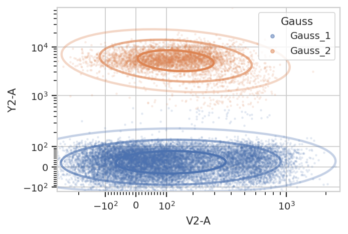
Basic usage, assigning each event to one of the mixture components: (the
isolines in the default_view() are 1, 2 and 3 standard deviations
away from the mean.)
g = flow.GaussianMixtureOp(name = "Gauss",
                           channels = ["V2-A", "Y2-A"],
                           scale = {"V2-A" : "logicle",
                                    "Y2-A" : "logicle"},
                           num_components = 2)
g.estimate(ex)
ex2 = g.apply(ex)
g.default_view().plot(ex2, alpha = 0.1)
/home/brian/src/cytoflow/cytoflow/operations/base_op_views.py:376: CytoflowViewWarning: Setting 'huefacet' to 'Gauss'

Subsetting based on standard deviation. Note: we use the Mahalnobis distance as a multivariate generalization of the number of standard deviations an event is from the mean of the multivariate gaussian.
g = flow.GaussianMixtureOp(name = "Gauss",
channels = ["V2-A", "Y2-A"],
scale = {"V2-A" : "logicle",
"Y2-A" : "logicle"},
num_components = 2,
sigma = 2)
g.estimate(ex)
ex2 = g.apply(ex)
g.default_view().plot(ex2, alpha = 0.1)
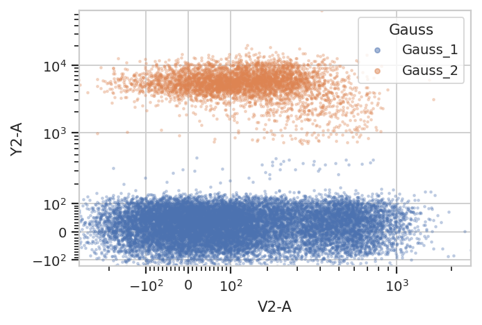
flow.ScatterplotView(xchannel = "V2-A",
ychannel = "Y2-A",
xscale = "logicle",
yscale = "logicle",
huefacet = "Gauss",
subset = "Gauss_1 == True | Gauss_2 == True").plot(ex2, alpha = 0.1)
/home/brian/src/cytoflow/cytoflow/operations/base_op_views.py:376: CytoflowViewWarning: Setting 'huefacet' to 'Gauss'

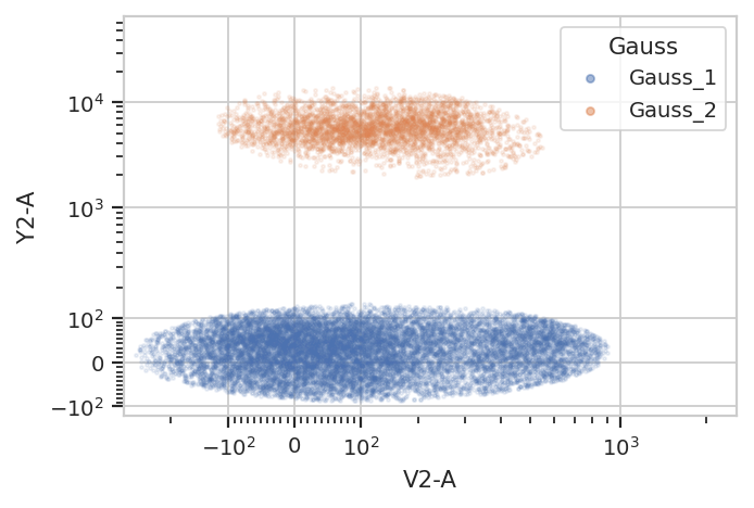
Gating based on posterior probabilities:
g = flow.GaussianMixtureOp(name = "Gauss",
                           channels = ["V2-A", "Y2-A"],
                           scale = {"V2-A" : "logicle",
                                    "Y2-A" : "logicle"},
                           num_components = 2,
                           posteriors = True)

g.estimate(ex)
ex2 = g.apply(ex)

g.default_view().plot(ex2, alpha = 0.1)

flow.ScatterplotView(xchannel = "V2-A",
                     ychannel = "Y2-A",
                     xscale = "logicle",
                     yscale = "logicle",
                     huefacet = "Gauss",
                     subset = "Gauss_1_posterior > 0.99 | Gauss_2_posterior > 0.99").plot(ex2)
/home/brian/src/cytoflow/cytoflow/operations/base_op_views.py:376: CytoflowViewWarning: Setting 'huefacet' to 'Gauss'
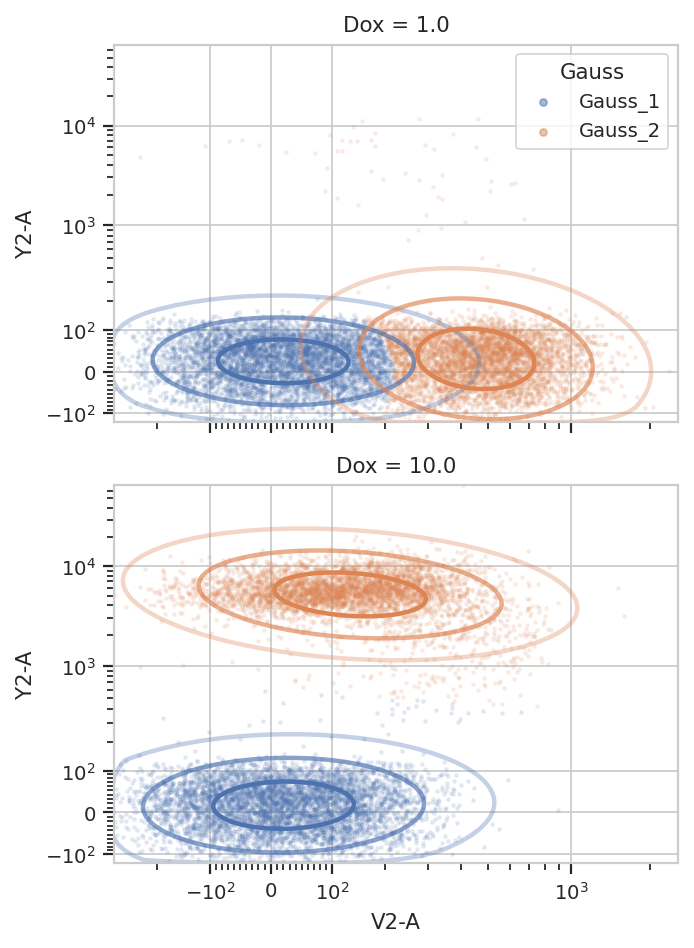
And multiple models for different subsets:
g = flow.GaussianMixtureOp(name = "Gauss",
                           channels = ["V2-A", "Y2-A"],
                           scale = {"V2-A" : "logicle",
                                    "Y2-A" : "logicle"},
                           num_components = 2,
                           by = ['Dox'])

g.estimate(ex)
ex2 = g.apply(ex)

g.default_view(yfacet = "Dox").plot(ex2, alpha = 0.1)
/home/brian/src/cytoflow/cytoflow/operations/base_op_views.py:376: CytoflowViewWarning: Setting 'huefacet' to 'Gauss'
Note that the new statistic has more columns – there are five for each channel.
ex2.statistics['Gauss']
| V2-A Mean | V2-A SD | V2-A Interval Low | V2-A Interval High | Y2-A Mean | Y2-A SD | Y2-A Interval Low | Y2-A Interval High | Proportion | ||
|---|---|---|---|---|---|---|---|---|---|---|
| Dox | Component | |||||||||
| 1.0 | 1 | 19.842218 | -162.552305 | -86.482396 | 129.557061 | 23.362101 | -65.458607 | -25.456763 | 75.287529 | 0.536379 |
| 2 | 451.472337 | -175.972193 | 273.492059 | 732.714475 | 28.819795 | -45.57717 | -38.813893 | 104.123691 | 0.463621 | |
| 10.0 | 1 | 20.283744 | -153.180224 | -94.385328 | 139.01489 | 16.076703 | -61.214443 | -36.784426 | 71.422587 | 0.559915 |
| 2 | 132.362846 | -142.924994 | 5.599064 | 295.121468 | 5144.549887 | -65.366477 | 3085.444584 | 8619.525681 | 0.440085 |
K-Means#
A gaussian mixture model can find clustered data, but it works best on
clusters that are shaped like gaussian distributions (duh). K-means
clustering is much more general. As with the GMM operation,
cytoflow’s K-means operation is N-dimensional and is parameterized
very similarly. Here’s a demonstration in 2D.
k = flow.KMeansOp(name = "KMeans",
                  channels = ["V2-A", "Y2-A"],
                  scale = {"V2-A" : "logicle",
                           "Y2-A" : "logicle"},
                  num_clusters = 2,
                  by = ['Dox'])

k.estimate(ex)
ex2 = k.apply(ex)
k.default_view(yfacet = "Dox").plot(ex2)
/home/brian/src/cytoflow/cytoflow/operations/base_op_views.py:376: CytoflowViewWarning: Setting 'huefacet' to 'KMeans'

Note how the centroids are marked with blue stars. The locations of the centroids and the proportion of events in each cluster are also saved as a new statistic:
ex2.statistics['KMeans']
| V2-A | Y2-A | Proportion | ||
|---|---|---|---|---|
| Dox | Cluster | |||
| 1.0 | 1 | 18.196680 | 27.874236 | 0.5302 |
| 2 | 469.188632 | 24.132975 | 0.4698 | |
| 10.0 | 1 | 128.942040 | 5146.910843 | 0.4409 |
| 2 | 20.614558 | 16.493200 | 0.5591 |
FlowPeaks#
Sometimes you want to cluster a data set and K-means just doesn’t work.
(It generally works best when clusters are fairly compact.) In such
cases, the unsupervized clustering algorithm flowPeaks may work
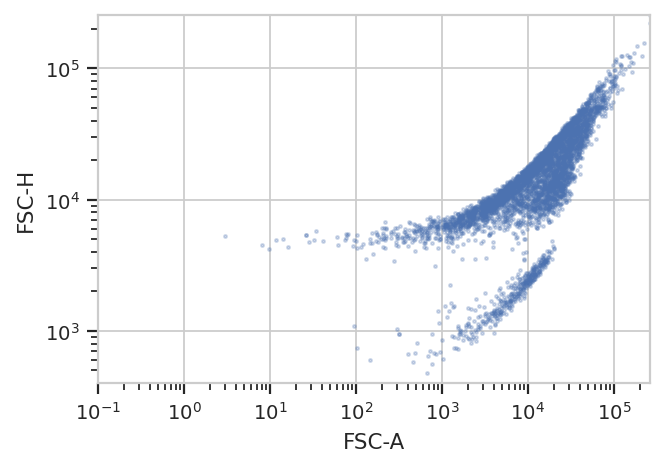
better for you. For example, the following FCS file (of an E. coli
experiment) shows clear separation between the cells (upper population)
and the particulate matter in the media (lower population.)
ex = flow.ImportOp(tubes = [flow.Tube(file = 'data/ecoli.fcs')]).apply()
flow.ScatterplotView(xchannel = "FSC-A",
                     xscale = 'log',
                     ychannel = "FSC-H",
                     yscale = 'log').plot(ex)
Unfortunately, K-means (even with more clusters than I want) isn’t finding them properly.
k = flow.KMeansOp(name = "KMeans",
                  channels = ["FSC-A", "FSC-H"],
                  scale = {"FSC-A" : "log",
                           "FSC-H" : "log"},
                  num_clusters = 3)

k.estimate(ex)
ex2 = k.apply(ex)
k.default_view().plot(ex2)
/home/brian/src/cytoflow/cytoflow/operations/base_op_views.py:376: CytoflowViewWarning: Setting 'huefacet' to 'KMeans'
flowPeaks is an unsupervized learning strategy developed
specifically for flow cytometry, and it works much better here. It
starts with a large number of (K-means) clusters, then makes “natural”
metaclusters – by doing so, it can automatically determine the number of
“natural” clusters in a data set. It is also much more computationally
expensive – if you have a large data set, be prepared to wait for a
while!
Another note – there are a number of hyperparameters for this method
that can dramatically change how it operates. The defaults are good for
many data sets; for the one below, I had to decrease h0 from 1.0
to 0.5. See the documentation for details. And note, even this
clustering isn’t perfect – there are a few events in a very minor
cluster, comprising 0.2% of the overall data set.
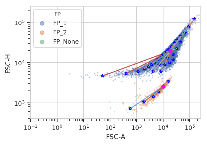
fp = flow.FlowPeaksOp(name = "FP",
channels = ["FSC-A", "FSC-H"],
scale = {"FSC-A" : "log",
"FSC-H" : "log"},
h0 = 0.5)
fp.estimate(ex)
ex2 = fp.apply(ex)
fp.default_view().plot(ex2)
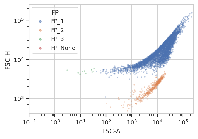
flow.ScatterplotView(xchannel = "FSC-A",
xscale = "log",
ychannel = "FSC-H",
yscale = "log",
huefacet = "FP").plot(ex2)
/home/brian/src/cytoflow/cytoflow/operations/base_op_views.py:376: CytoflowViewWarning: Setting 'huefacet' to 'FP'
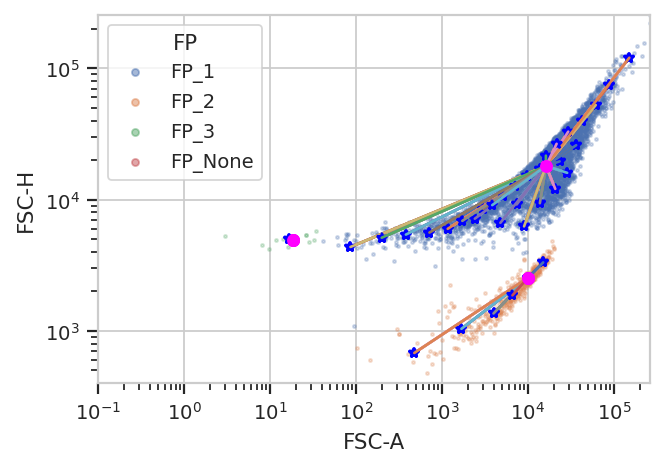
The new statistic is similar to the one added by KMeansOp – a column
for each channel, saying where the metaclusters’ centers were, and a
column saying the proportion of events in each cluster.
ex2.statistics['FP']
| FSC-A | FSC-H | Proportion | |
|---|---|---|---|
| Cluster | |||
| 1 | 16233.769453 | 18064.409717 | 0.8256 |
| 2 | 9943.351666 | 2531.893295 | 0.0778 |
| 3 | 18.550837 | 4906.887351 | 0.0022 |