cytoflow.operations.tsne

Apply t-Distributed Stochastic Neighbor Embedding (tSNE) to flow data. This is similar to principle component analysis, in that it is a dimensionality reduction algorithm. Unlike PCA, it is non-linear and (supposedly) retains internal structure better than PCA. tsne has one class:

tSNEOp – the IOperation that applies tSNE to an Experiment.

class cytoflow.operations.tsne.tSNEOp

Bases: HasStrictTraits

Use t-Distributed Stochastic Neighbor Embedding to reduce the dimensionality of the data set.

Call estimate to compute the embedding.

Calling apply creates new “channels” named {name}_1 and {name}_2, where name is the name attribute. (Unlike PCA, tSNE only decomposes to two components.)

The same decomposition may not be appropriate for different subsets of the data set. If this is the case, you can use the by attribute to specify metadata by which to aggregate the data before estimating (and applying) a model. The tSNE parameters such as the perplexity are the same across each subset, though

name

The operation name; determines the name of the new columns.

Type:

Str

channels

The channels to apply the decomposition to.

Type:

List(Str)

scale

Re-scale the data in the specified channels before fitting. If a channel is in channels but not in scale, the current package-wide default (set with set_default_scale) is used.

Type:

Dict(Str : {“linear”, “logicle”, “log”})

by

A list of metadata attributes to aggregate the data before estimating the model. For example, if the experiment has two pieces of metadata, Time and Dox, setting by to ["Time", "Dox"] will fit the model separately to each subset of the data with a unique combination of Time and Dox.

Type:

List(Str)

metric

How to compute “distance”? If using many channels, try changing to cosine.

Type:

Enum(“euclidean”, “cosine”) (default = “euclidian”)

perplexity

The balance between the local and global structure of the data. Larger datasets benefit from higher perplexity, but be warned – runtime scales linearly with perplexity!

Type:

Float (default = 10)

sample

What proportion of the data set to use for training? Defaults to 1% of the dataset to help with runtime.

Type:

Float (default = 0.01)

Notes

Uses openTSNE by Pavlin G. Policar, Martin Strazar and Blaz Zupan [1]

References

[1]

Poliar, PG and Strazar, M and Zupan, Blaz (2024). openTSNE: A Modular Python Library for t-SNE Dimensionality Reduction and Embedding Journal of Statistical Software 109: 1-30. https://www.jstatsoft.org/index.php/jss/article/view/v109i03

Examples

Make a little data set.

>>> import cytoflow as flow
>>> import_op = flow.ImportOp()
>>> import_op.tubes = [flow.Tube(file = "Plate01/RFP_Well_A3.fcs",
...                              conditions = {'Dox' : 10.0}),
...                    flow.Tube(file = "Plate01/CFP_Well_A4.fcs",
...                              conditions = {'Dox' : 1.0})]
>>> import_op.conditions = {'Dox' : 'float'}
>>> ex = import_op.apply()

Create and parameterize the operation.

>>> tsne = flow.tSNEOp(name = 'tSNE',
...                    channels = ['V2-A', 'V2-H', 'Y2-A', 'Y2-H'],
...                    scale = {'V2-A' : 'log',
...                             'V2-H' : 'log',
...                             'Y2-A' : 'log',
...                             'Y2-H' : 'log'},
...                    by = ["Dox"])

Estimate the decomposition

>>> tsne.estimate(ex)

Apply the operation

>>> ex2 = tsne.apply(ex)

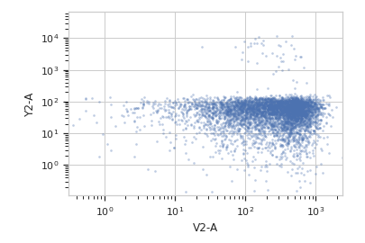
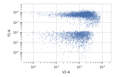
Plot a scatterplot of the decomposition. Compare to a scatterplot of the underlying channels.

>>> flow.ScatterplotView(xchannel = "V2-A",
...                      xscale = "log",
...                      ychannel = "Y2-A",
...                      yscale = "log",
...                      subset = "Dox == 1.0").plot(ex2)

>>> flow.ScatterplotView(xchannel = "tSNE_1",
...                      ychannel = "tSNE_2",
...                      subset = "Dox == 1.0").plot(ex2)

>>> flow.ScatterplotView(xchannel = "V2-A",
...                      xscale = "log",
...                      ychannel = "Y2-A",
...                      yscale = "log",
...                      subset = "Dox == 10.0").plot(ex2)

>>> flow.ScatterplotView(xchannel = "tSNE_1",
...                      ychannel = "tSNE_2",
...                      subset = "Dox == 10.0").plot(ex2)

estimate(experiment, subset=None)

Estimate the decomposition

Parameters:

• experiment (Experiment) – The Experiment to use to estimate the k-means clusters

• subset (str (default = None)) – A Python expression that specifies a subset of the data in experiment to use to parameterize the operation.

apply(experiment)

Apply the tSNE decomposition to the data.

Returns:

a new Experiment with additional Experiment.channels named name_1 and name_2

Return type:

Experiment