Statistics in cytoflow#
One of the most powerful concepts in cytoflow is that it makes it
easy to summarize your data, then track how those summaries change as
your experimental variables change. This notebook demonstrates several
different modules that create and plot statistics.
Import the cytoflow module.
import cytoflow as flow

# if your figures are too big or too small, you can scale them by changing matplotlib's DPI
import matplotlib
matplotlib.rc('figure', dpi = 160)
We use the same data set as the Yeast Dose Response example notebook, with one variant: we load each tube three times, grabbing only 100 events from each.
inputs = {
    "Yeast_B1_B01.fcs" : 5.0,
    "Yeast_B2_B02.fcs" : 3.75,
    "Yeast_B3_B03.fcs" : 2.8125,
    "Yeast_B4_B04.fcs" : 2.109,
    "Yeast_B5_B05.fcs" : 1.5820,
    "Yeast_B6_B06.fcs" : 1.1865,
    "Yeast_B7_B07.fcs" : 0.8899,
    "Yeast_B8_B08.fcs" : 0.6674,
    "Yeast_B9_B09.fcs" : 0.5,
    "Yeast_B10_B10.fcs" : 0.3754,
    "Yeast_B11_B11.fcs" : 0.2816,
    "Yeast_B12_B12.fcs" : 0.2112,
    "Yeast_C1_C01.fcs" : 0.1584,
    "Yeast_C2_C02.fcs" : 0.1188,
    "Yeast_C3_C03.fcs" : 0.0892,
    "Yeast_C4_C04.fcs" : 0.0668,
    "Yeast_C5_C05.fcs" : 0.05,
    "Yeast_C6_C06.fcs" : 0.0376,
    "Yeast_C7_C07.fcs" : 0.0282,
    "Yeast_C8_C08.fcs" : 0.0211,
    "Yeast_C9_C09.fcs" : 0.0159
}

tubes = []
for filename, ip in inputs.items():
    tubes.append(flow.Tube(file = "data/" + filename, conditions = {'IP' : ip, 'Replicate' : 1}))
    tubes.append(flow.Tube(file = "data/" + filename, conditions = {'IP' : ip, 'Replicate' : 2}))
    tubes.append(flow.Tube(file = "data/" + filename, conditions = {'IP' : ip, 'Replicate' : 3}))


ex = flow.ImportOp(conditions = {'IP' : "float", "Replicate" : "int"},
                   tubes = tubes,
                   events = 100).apply()
In cytoflow, a statistic is a value that summarizes something
about some data. cytoflow makes it easy to compute statistics for
various subsets. For example, if we expect the geometric mean of
FITC-A channel to change as the IP variable changes, we can
compute the geometric mean of the FITC-A channel of each different
IP condition with the ChannelStatisticOp operation:
op = flow.ChannelStatisticOp(name = "ByIP",
                             by = ["IP"],
                             channel = "FITC-A",
                             function = flow.geom_mean)
ex2 = op.apply(ex)
This operation splits the data set by different values of IP, then
applies the function flow.geom_mean to the FITC-A channel in
each subset. The result is stored in the statistics attribute of an
Experiment. The statistics attribute is a dictionary whose keys
are the names of the operations that added the statistics:
ex2.statistics.keys()
dict_keys(['Conditions', 'ByIP'])
The value of each entry in Experiment.statistics is a
pandas.DataFrame whose index is all the subsets for which the
statistic was computed, and the contents are the values of the statstic
itself. ImportOp stores a statistic called Conditions – it’s the
conditions of each tube we loaded – and ByIP is the statistic we
just computed.
ex2.statistics['ByIP']
| FITC-A | |
|---|---|
| IP | |
| 0.0159 | 110.689216 |
| 0.0211 | 145.457491 |
| 0.0282 | 158.179844 |
| 0.0376 | 191.686432 |
| 0.0500 | 247.427608 |
| 0.0668 | 429.696322 |
| 0.0892 | 671.304186 |
| 0.1188 | 928.771756 |
| 0.1584 | 1190.565628 |
| 0.2112 | 1155.330712 |
| 0.2816 | 1581.640661 |
| 0.3754 | 1720.358247 |
| 0.5000 | 1908.171933 |
| 0.6674 | 2275.226081 |
| 0.8899 | 2338.875702 |
| 1.1865 | 2511.012014 |
| 1.5820 | 2438.501368 |
| 2.1090 | 2414.304459 |
| 2.8125 | 2606.973466 |
| 3.7500 | 2750.040554 |
| 5.0000 | 2229.964776 |
We can also specify multiple variables to break data set into. In the
example above, Statistics1DOp lumps all events with the same value
of IP together, but each amount of IP actually has three values
of Replicate as well. Let’s apply geom_mean to each unique
combination of IP and Replicate:
op = flow.ChannelStatisticOp(name = "ByIP",
                             by = ["IP", "Replicate"],
                             channel = "FITC-A",
                             function = flow.geom_mean)
ex2 = op.apply(ex)
ex2.statistics["ByIP"][0:12]
| FITC-A | ||
|---|---|---|
| IP | Replicate | |
| 0.0159 | 1 | 102.937468 |
| 2 | 115.299550 | |
| 3 | 114.317690 | |
| 0.0211 | 1 | 136.798600 |
| 2 | 146.395310 | |
| 3 | 153.673670 | |
| 0.0282 | 1 | 151.769626 |
| 2 | 159.617006 | |
| 3 | 163.376433 | |
| 0.0376 | 1 | 193.639169 |
| 2 | 193.623095 | |
| 3 | 187.855429 |
Note that the pandas.DataFrame now has a MultiIndex: there are
values for each unique combination of IP and Replicate.
Now that we have computed a statistic, we can plot it with one of the statistics views. We can use a bar chart:
flow.BarChartView(statistic = "ByIP",
                  feature = "FITC-A",
                  variable = "IP").plot(ex2)
---------------------------------------------------------------------------

CytoflowViewError                         Traceback (most recent call last)

Cell In[7], line 3
      1 flow.BarChartView(statistic = "ByIP",
      2                   feature = "FITC-A",
----> 3                   variable = "IP").plot(ex2)


File ~/src/cytoflow/cytoflow/views/bar_chart.py:134, in BarChartView.plot(self, experiment, plot_name, **kwargs)
    108 def plot(self, experiment, plot_name = None, **kwargs):
    109     """
    110     Plot a bar chart
    111
   (...)    131
    132     """
--> 134     super().plot(experiment, plot_name, **kwargs)


File ~/src/cytoflow/cytoflow/views/base_views.py:973, in Base1DStatisticsView.plot(self, experiment, plot_name, **kwargs)
    962     raise util.CytoflowViewError('variable',
    963                                  "variable {0} not in the experiment"
    964                             .format(self.variable))
    966 scale = util.scale_factory(self.scale,
    967                            experiment,
    968                            statistic = self.statistic,
    969                            features = [self.feature]
    970                                         + ([self.error_high] if self.error_high else [])
    971                                         + ([self.error_low] if self.error_low else []))
--> 973 super().plot(experiment,
    974              plot_name = plot_name,
    975              scale = scale,
    976              **kwargs)


File ~/src/cytoflow/cytoflow/views/base_views.py:824, in BaseStatisticsView.plot(self, experiment, plot_name, **kwargs)
    821 groupby = data.groupby(unused_names, observed = True)
    823 if plot_name is None:
--> 824     raise util.CytoflowViewError('plot_name',
    825                                  "You must use facets {} in either the "
    826                                  "plot variables or the plot name. "
    827                                  "Possible plot names: {}"
    828                                  .format(unused_names, list(groupby.groups.keys())))
    830 if plot_name not in set(groupby.groups.keys()):
    831     raise util.CytoflowViewError('plot_name',
    832                                  "plot_name must be one of {}"
    833                                  .format(plot_name, list(groupby.groups.keys())))


CytoflowViewError: ('plot_name', "You must use facets ['Replicate'] in either the plot variables or the plot name. Possible plot names: [1, 2, 3]")
Oops! We forgot to specify how to plot the different Replicates.
Each index of a statistic must be specified as either a variable or a
facet of the plot, like so:
flow.BarChartView(statistic = "ByIP",
                  feature = "FITC-A",
                  variable = "IP",
                  huefacet = "Replicate").plot(ex2)

Note that because a statistic can contain multiple columns, we have to
specify which one of them to plot. Taking a term from machine learning,
cytoflow calls each column of a statistic a feature. Thus,
feature = "FITC-A" tells the BarChartView to plot the FITC-A
column of the statistic. By default, ChannelStatisticOp creates a
statistic with one feature, named the same as the channel the function
was applied to. However, if your function returns a pandas.Series,
the row names of the series become the column names.
A quick aside - sometimes you get ugly axes because of overlapping
labels. In this case, we want a wider plot. While we can directly
specify the height of a plot, we can’t directly specify its width, only
its aspect ratio (the ratio of the width to the height.) cytoflow
defaults to 1.5; in this case, let’s widen it out to 4. If this results
in a plot that’s wider than your browser, the Jupyter notebook will
scale it down for you.
flow.BarChartView(statistic = "ByIP",
                  feature = "FITC-A",
                  variable = "IP",
                  huefacet = "Replicate").plot(ex2, aspect = 4)

Bar charts are really best for categorical variables (with a modest number of categories.) Let’s do a line chart instead:
flow.Stats1DView(statistic = "ByIP",
                 feature = "FITC-A",
                 variable = "IP",
                 variable_scale = 'log',
                 huefacet = "Replicate").plot(ex2)

1D and 2D statistics views can also plot error bars; the high and low
values must be features in the same statistic, which is pretty easy to
do if the function you use in ChannelStatisticOp returns a
pandas.Series. Here’s an example that uses a lambda expression to
avoid defining a whole new function, computing the geometric mean and
standard deviation of each subset:
# While an arithmetic SD is usually plotted plus-or-minus the arithmetic mean,
# a *geometric* SD is usually plotted (on a log scale!) multiplied-or-divided by the
# geometric mean.  the function geom_sd_range is a convenience function that does this.

import pandas as pd
ex2 = flow.ChannelStatisticOp(name = "ByIP",
                              by = ["IP"],
                              channel = "FITC-A",
                              function = lambda x: pd.Series({"Geo.Mean" : flow.geom_mean(x),
                                                              "*SD" : flow.geom_mean(x) * flow.geom_sd(x),
                                                              "/SD" : flow.geom_mean(x) / flow.geom_sd(x)})).apply(ex)

flow.Stats1DView(statistic = "ByIP",
                 variable = "IP",
                 variable_scale = "log",
                 feature = "Geo.Mean",
                 scale = "log",
                 error_low = "/SD",
                 error_high = "*SD").plot(ex2, shade_error = True)

The plot above shows how one statistic varies (on the Y axis) as a
variable changes on the X axis. It also demonstrates that we can control
the visual aspects of the plot by the parameters passed to plot().
The rule-of-thumb to remember is that the view object’s attributes
determine what is plotted; the parameters passed to plot() determine
how it is plotted. We pass many of these parameters straight through
to the underlying seaborn and matplotlib plotting functions; see
the documentation of each view for details.
We can also plot two features against eachother, one on the X axis and one on the Y axis. For example, we can ask if the geometric standard deviation varies as the geometric mean changes:
ex2 = flow.ChannelStatisticOp(name = "ByIP",
                              by = ["IP"],
                              channel = "FITC-A",
                              function = lambda x: pd.Series({"Geo.Mean" : flow.geom_mean(x),
                                                              "Geo.SD" : flow.geom_sd(x)})).apply(ex)

flow.Stats2DView(statistic = "ByIP",
                 variable = "IP",
                 xfeature = "Geo.Mean",
                 yfeature = "Geo.SD",
                 yscale = "log").plot(ex2)
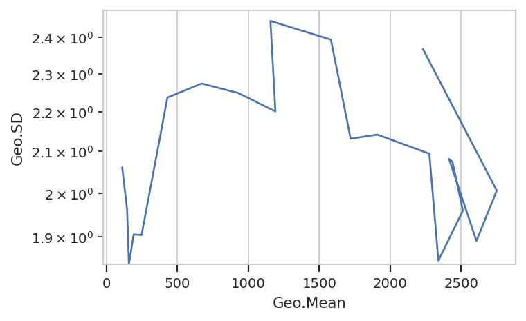
Nope, guess not. See the TASBE Calibrated Flow Cytometry notebook for more examples of 1D and 2D statistics views.
Transforming statistics#
In addition to making statistics by applying summary functions to data,
you can also apply functions to other statistics. For example, a common
question is “What percentage of my events are in a particular gate?” We
could, for instance, ask what percentage of events are above 1000 in the
FITC-A channel, and how that varies by amount of IP. We start by
defining a threshold gate with ThresholdOp:
thresh = flow.ThresholdOp(name = "Above1000",
                          channel = "FITC-A",
                          threshold = 1000)
ex2 = thresh.apply(ex)
Now, the Experiment has a condition named Above1000 that is
True or False depending on whether that event’s FITC-A
channel is greater than 1000. Next, we compute the total number of
events in each subset with a unique combination of Above1000 and
IP:
ex3 = flow.ChannelStatisticOp(name = "Above1000",
                              by = ["Above1000", "IP"],
                              channel = "FITC-A",
                              function = len).apply(ex2)
ex3.statistics["Above1000"]
| FITC-A | ||
|---|---|---|
| Above1000 | IP | |
| False | 0.0159 | 300.0 |
| 0.0211 | 298.0 | |
| 0.0282 | 300.0 | |
| 0.0376 | 299.0 | |
| 0.0500 | 296.0 | |
| 0.0668 | 255.0 | |
| 0.0892 | 199.0 | |
| 0.1188 | 150.0 | |
| 0.1584 | 105.0 | |
| 0.2112 | 100.0 | |
| 0.2816 | 66.0 | |
| 0.3754 | 65.0 | |
| 0.5000 | 52.0 | |
| 0.6674 | 28.0 | |
| 0.8899 | 19.0 | |
| 1.1865 | 21.0 | |
| 1.5820 | 27.0 | |
| 2.1090 | 25.0 | |
| 2.8125 | 14.0 | |
| 3.7500 | 11.0 | |
| 5.0000 | 32.0 | |
| True | 0.0211 | 2.0 |
| 0.0376 | 1.0 | |
| 0.0500 | 4.0 | |
| 0.0668 | 45.0 | |
| 0.0892 | 101.0 | |
| 0.1188 | 150.0 | |
| 0.1584 | 195.0 | |
| 0.2112 | 200.0 | |
| 0.2816 | 234.0 | |
| 0.3754 | 235.0 | |
| 0.5000 | 248.0 | |
| 0.6674 | 272.0 | |
| 0.8899 | 281.0 | |
| 1.1865 | 279.0 | |
| 1.5820 | 273.0 | |
| 2.1090 | 275.0 | |
| 2.8125 | 286.0 | |
| 3.7500 | 289.0 | |
| 5.0000 | 268.0 |
And now we compute the proportion of Above1000 == True for each
value of IP. TransformStatisticOp applies a function to subsets
of a statistic – the function must take a single pandas.Series
parameter and it may return either a single float value, in which
case the operation is a reduction, or it may return a pandas.Series
whose row names become the new column names of the new statistic, or it
can return a pandas.Series with the same index as the passed series,
in which case it is a transformation. (In this last case, leave by
unset.) Here, we’re applying a lambda function to convert each
IP subset from length into proportion.
import pandas as pd

ex4 = flow.TransformStatisticOp(name = "PropAbove1000",
                                statistic = "Above1000",
                                feature = "FITC-A",
                                by = ["IP"],
                                function = lambda a: a / a.sum()).apply(ex3)
---------------------------------------------------------------------------

CytoflowOpError                           Traceback (most recent call last)

Cell In[15], line 7
      1 import pandas as pd
      3 ex4 = flow.TransformStatisticOp(name = "PropAbove1000",
      4                                 statistic = "Above1000",
      5                                 feature = "FITC-A",
      6                                 by = ["IP"],
----> 7                                 function = lambda a: a / a.sum()).apply(ex3)
      9 ex4.statistics["PropAbove1000"][0:8]


File ~/src/cytoflow/cytoflow/operations/xform_stat.py:324, in TransformStatisticOp.apply(self, experiment)
    322         elif isinstance(v, pd.Series):
    323             if not v.index.equals(first_v.index):
--> 324                 raise util.CytoflowOpError('function',
    325                                            "The first call of 'function' returned series with index of {}, "
    326                                            "but the call on group {} returned a series with index {}. "
    327                                            "All returned series must have the same index!"
    328                                            .format(first_v.index, group, v.index))
    329         new_stat.loc[group] = v
    331         # # check for, and warn about, NaNs.
    332         # if np.any(np.isnan(new_stat.loc[group])):
    333         #     raise util.CytoflowOpError('function',
   (...)    336
    337 else:


CytoflowOpError: ('function', "The first call of 'function' returned series with index of Index([False], dtype='bool', name='Above1000'), but the call on group (0.0211,) returned a series with index Index([False, True], dtype='bool', name='Above1000'). All returned series must have the same index!")
That’s a pretty ugly error – but the cause is straightforward. Look at
the values in the statistic above and notice how there is an entry for
Above1000 == False, IP == 0.0159 but there isn’t a corresponding
entry for Above1000 == True, IP == 0.0159? When we called
a / a.sum() on the subset of the statistic with IP == 0.0159, it
returned a Series with only one row – False. However, when we
did the same function on the subset of the statistic with
IP == 0.0211, now that subset has two rows, False and True –
and when we compute a / a.sum(), we get a Series that similarly
has two rows.
This is a not uncommon situation. You can solve it by setting
ignore_incomplete_groups to True.
ex4 = flow.TransformStatisticOp(name = "PropAbove1000",
                                statistic = "Above1000",
                                feature = "FITC-A",
                                by = ["IP"],
                                function = lambda a: a / a.sum(),
                                ignore_incomplete_groups = True).apply(ex3)

ex4.statistics["PropAbove1000"][0:8]
| False | True | |
|---|---|---|
| IP | ||
| 0.0211 | 0.993333 | 0.006667 |
| 0.0376 | 0.996667 | 0.003333 |
| 0.0500 | 0.986667 | 0.013333 |
| 0.0668 | 0.850000 | 0.150000 |
| 0.0892 | 0.663333 | 0.336667 |
| 0.1188 | 0.500000 | 0.500000 |
| 0.1584 | 0.350000 | 0.650000 |
| 0.2112 | 0.333333 | 0.666667 |
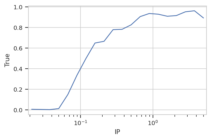
Note that because our lambda function returns a small pandas.Series
with rows named False and True, the columns in our new statistic
are also named False and True. Now we can plot the True
column of the new statistic.
flow.Stats1DView(statistic = "PropAbove1000",
                 feature = "True",
                 variable = "IP",
                 variable_scale = "log").plot(ex4)
Statistics from data-driven modules#
One of the most exciting aspects of statistics in cytoflow is that
other data-driven modules can add them to an Experiment, too. Let’s
look at a quick example, starting by re-loading the entire yeast
induction dataset:
import cytoflow as flow
inputs = {
    "Yeast_B1_B01.fcs" : 5.0,
    "Yeast_B2_B02.fcs" : 3.75,
    "Yeast_B3_B03.fcs" : 2.8125,
    "Yeast_B4_B04.fcs" : 2.109,
    "Yeast_B5_B05.fcs" : 1.5820,
    "Yeast_B6_B06.fcs" : 1.1865,
    "Yeast_B7_B07.fcs" : 0.8899,
    "Yeast_B8_B08.fcs" : 0.6674,
    "Yeast_B9_B09.fcs" : 0.5,
    "Yeast_B10_B10.fcs" : 0.3754,
    "Yeast_B11_B11.fcs" : 0.2816,
    "Yeast_B12_B12.fcs" : 0.2112,
    "Yeast_C1_C01.fcs" : 0.1584,
    "Yeast_C2_C02.fcs" : 0.1188,
    "Yeast_C3_C03.fcs" : 0.0892,
    "Yeast_C4_C04.fcs" : 0.0668,
    "Yeast_C5_C05.fcs" : 0.05,
    "Yeast_C6_C06.fcs" : 0.0376,
    "Yeast_C7_C07.fcs" : 0.0282,
    "Yeast_C8_C08.fcs" : 0.0211,
    "Yeast_C9_C09.fcs" : 0.0159
}

tubes = []
for filename, ip in inputs.items():
    tubes.append(flow.Tube(file = "data/" + filename, conditions = {'IP' : ip}))


ex = flow.ImportOp(conditions = {'IP' : "float"},
                   tubes = tubes).apply()
For this example, we’ll use the GaussianMixtureOp operation. It adds
a statistic for each component of the mixture model it fits, containing
the mean, standard deviation, and a few other statistics (see the docs
for details):
op = flow.GaussianMixtureOp(name = "Gauss",
                            channels = ["FITC-A"],
                            scale = {"FITC-A" : 'logicle'},
                            by = ["IP"],
                            num_components = 1)
op.estimate(ex)
ex2 = op.apply(ex)
ex2.statistics["Gauss"]
| FITC-A Mean | FITC-A SD | FITC-A Interval Low | FITC-A Interval High | ||
|---|---|---|---|---|---|
| IP | Component | ||||
| 0.0159 | 1 | 114.867593 | 6.044478 | 56.944599 | 224.178352 |
| 0.0211 | 1 | 146.760865 | 3.206172 | 80.365347 | 265.784241 |
| 0.0282 | 1 | 161.831942 | 3.483374 | 88.275085 | 295.421818 |
| 0.0376 | 1 | 188.241811 | 4.164093 | 101.184975 | 350.418214 |
| 0.0500 | 1 | 252.533895 | 6.484476 | 127.952042 | 502.065649 |
| 0.0668 | 1 | 415.359435 | 9.197695 | 195.235139 | 894.571209 |
| 0.0892 | 1 | 675.335896 | 9.728315 | 310.618328 | 1484.661773 |
| 0.1188 | 1 | 976.574632 | 10.505229 | 437.615067 | 2200.01757 |
| 0.1584 | 1 | 1212.127491 | 10.465049 | 542.10246 | 2732.441099 |
| 0.2112 | 1 | 1169.357113 | 15.521608 | 459.268595 | 3011.330277 |
| 0.2816 | 1 | 1491.938821 | 14.379383 | 601.114014 | 3736.10692 |
| 0.3754 | 1 | 1683.611714 | 8.79359 | 784.03122 | 3635.893765 |
| 0.5000 | 1 | 1812.128528 | 10.671024 | 802.324829 | 4117.843047 |
| 0.6674 | 1 | 2233.860489 | 5.486517 | 1134.295446 | 4414.715041 |
| 0.8899 | 1 | 2341.076532 | 3.721475 | 1246.733302 | 4408.71647 |
| 1.1865 | 1 | 2474.300525 | 5.4483 | 1256.858649 | 4886.579643 |
| 1.5820 | 1 | 2401.710245 | 7.58679 | 1151.729762 | 5027.751372 |
| 2.1090 | 1 | 2383.285932 | 6.973761 | 1161.983753 | 4906.469724 |
| 2.8125 | 1 | 2411.122019 | 3.921717 | 1276.836189 | 4566.134877 |
| 3.7500 | 1 | 2584.007182 | 6.44288 | 1277.360041 | 5244.721547 |
| 5.0000 | 1 | 2265.732416 | 8.988694 | 1046.899394 | 4925.741101 |
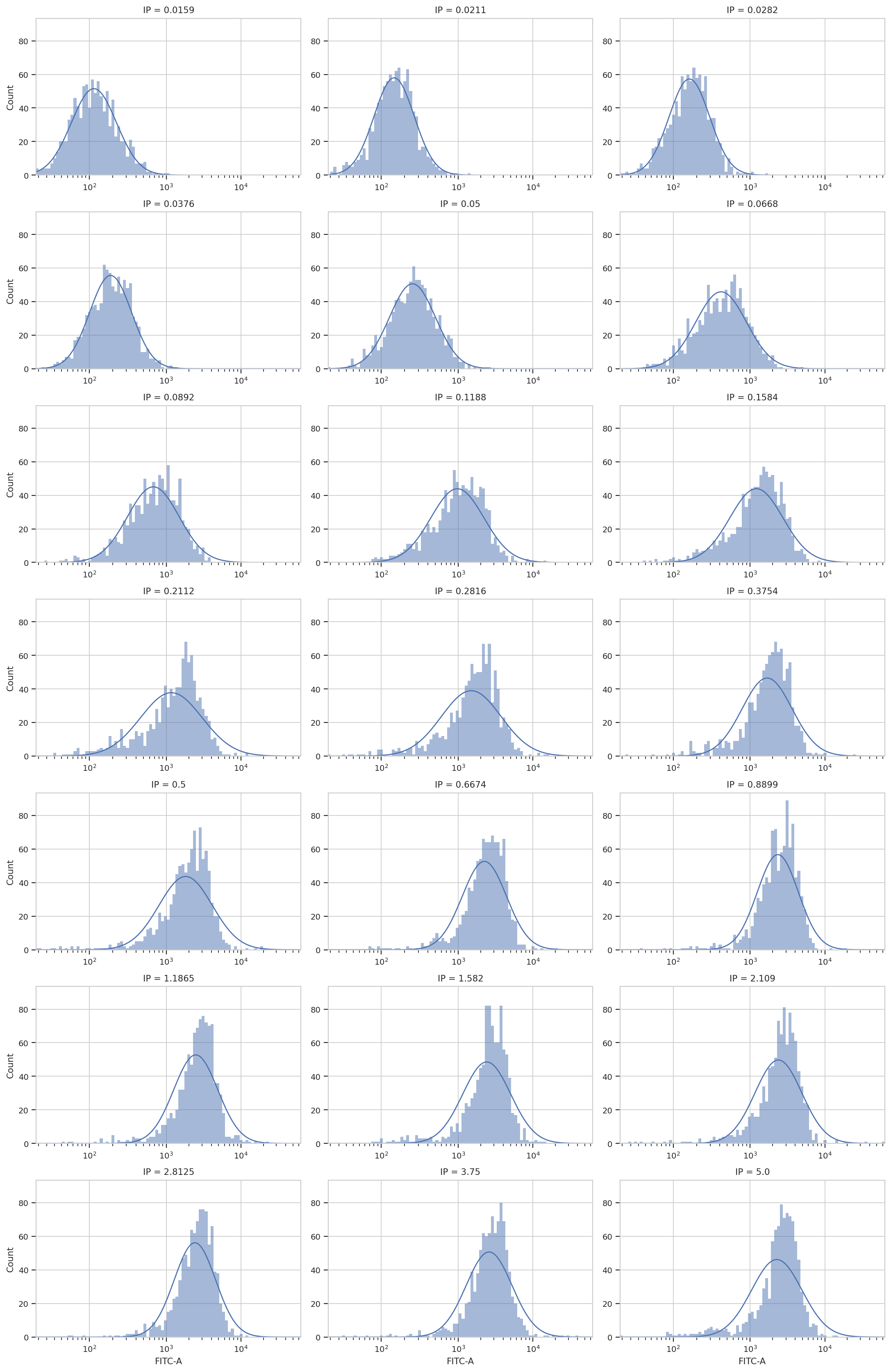
Many operations also have a “default” view which provides more
information about how they ran. For example, the GaussianMixtureOp
class has a default_view() member that returns a view which plots
the underlying data as well as the gaussian curves that were fit:
op.default_view(xfacet = "IP").plot(ex2, col_wrap = 3)
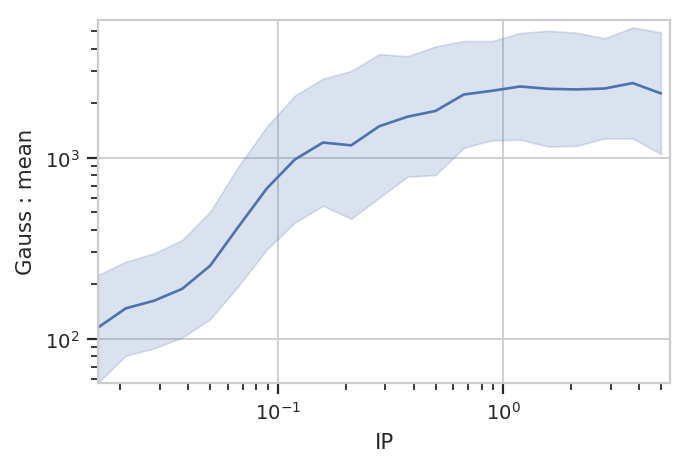
Let’s plot the mean as it varies with IP concentration, along with the interval +/- one standard deviation:
flow.Stats1DView(statistic = "Gauss",
                 feature = "FITC-A Mean",
                 variable = "IP",
                 variable_scale = "log",
                 scale = "log",
                 error_low = "FITC-A Interval Low",
                 error_high = "FITC-A Interval High").plot(ex2, shade_error = True)
/home/brian/src/cytoflow/cytoflow/views/base_views.py:862: CytoflowViewWarning: Only one value for level Component; dropping it.