cytoflow.operations.density#
The density module has two classes:
DensityGateOp – gates an Experiment based on a
two-dimensional (smoothed) density plot.
DensityGateView – diagnostic view that plots the gate
estimated by the DensityGateOp.
- class cytoflow.operations.density.DensityGateOp[source]#
Bases:
HasStrictTraitsThis module computes a gate based on a 2D density plot. The user chooses what proportion of events to keep, and the module creates a gate that selects that proportion of events in the highest-density bins of the 2D density histogram.
- name#
The operation name; determines the name of the new metadata column
- Type:
Str
- xchannel#
The X channel to apply the binning to.
- Type:
Str
- ychannel#
The Y channel to apply the binning to.
- Type:
Str
- xscale#
Re-scale the data on the X acis before fitting the data?
- Type:
{“linear”, “logicle”, “log”} (default = “linear”)
- yscale#
Re-scale the data on the Y axis before fitting the data?
- Type:
{“linear”, “logicle”, “log”} (default = “linear”)
- keep#
What proportion of events to keep? Must be
>0and<1- Type:
Float (default = 0.9)
- bins#
How many bins should there be on each axis? Must be positive.
- Type:
Int (default = 100)
- min_quantile#
Clip values below this quantile
- Type:
Float (default = 0.001)
- max_quantile#
Clip values above this quantile
- Type:
Float (default = 1.0)
- sigma#
What standard deviation to use for the gaussian blur?
- Type:
Float (default = 1.0)
- by#
A list of metadata attributes to aggregate the data before estimating the gate. For example, if the experiment has two pieces of metadata,
TimeandDox, settingby = ["Time", "Dox"]will fit a separate gate to each subset of the data with a unique combination ofTimeandDox.- Type:
List(Str)
Notes
This gating method was developed by John Sexton, in Jeff Tabor’s lab at Rice University.
From http://taborlab.github.io/FlowCal/fundamentals/density_gate.html, the method is as follows:
Determines the number of events to keep, based on the user specified gating fraction and the total number of events of the input sample.
Divides the 2D channel space into a rectangular grid, and counts the number of events falling within each bin of the grid. The number of counts per bin across all bins comprises a 2D histogram, which is a coarse approximation of the underlying probability density function.
Smoothes the histogram generated in Step 2 by applying a Gaussian Blur. Theoretically, the proper amount of smoothing results in a better estimate of the probability density function. Practically, smoothing eliminates isolated bins with high counts, most likely corresponding to noise, and smoothes the contour of the gated region.
Selects the bins with the greatest number of events in the smoothed histogram, starting with the highest and proceeding downward until the desired number of events to keep, calculated in step 1, is achieved.
Examples
Make a little data set.
>>> import cytoflow as flow
>>> import_op = flow.ImportOp()
>>> import_op.tubes = [flow.Tube(file = "Plate01/RFP_Well_A3.fcs",
...                              conditions = {'Dox' : 10.0}),
...                    flow.Tube(file = "Plate01/CFP_Well_A4.fcs",
...                              conditions = {'Dox' : 1.0})]
>>> import_op.conditions = {'Dox' : 'float'}
>>> ex = import_op.apply()
Create and parameterize the operation.
>>> dens_op = flow.DensityGateOp(name = 'Density',
...                              xchannel = 'FSC-A',
...                              xscale = 'log',
...                              ychannel = 'SSC-A',
...                              yscale = 'log',
...                              keep = 0.5)
Find the bins to keep
>>> dens_op.estimate(ex)
Plot a diagnostic view
>>> dens_op.default_view().plot(ex)
Apply the gate
>>> ex2 = dens_op.apply(ex)
- estimate(experiment, subset=None)[source]#
Split the data set into bins and determine which ones to keep.
- Parameters:
experiment (
Experiment) – TheExperimentto use to estimate the gate parameters.subset (Str (default = None)) – If set, determine the gate parameters on only a subset of the
experimentparameter.
- apply(experiment)[source]#
Creates a new condition based on membership in the gate that was parameterized with
estimate.- Parameters:
experiment (
Experiment) – theExperimentto apply the gate to.- Returns:
a new
Experimentwith the new gate applied.- Return type:
- default_view(**kwargs)[source]#
Returns a diagnostic plot of the Gaussian mixture model.
- Returns:
a diagnostic view, call
DensityGateView.plotto see the diagnostic plot.- Return type:
- class cytoflow.operations.density.DensityGateView[source]#
Bases:
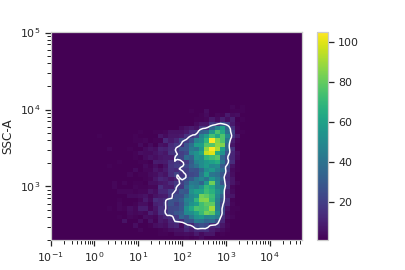
By2DView,AnnotatingView,DensityViewA diagnostic view for
DensityGateOp. Draws a density plot, then outlines the selected bins in white.- facets#
A read-only list of the conditions used to facet this view.
- Type:
List(Str)
- by#
A read-only list of the conditions used to group this view’s data before plotting.
- Type:
List(Str)
- xchannel#
The channels to use for this view’s X axis. If you created the view using
default_view, this is already set.- Type:
Str
- ychannel#
The channels to use for this view’s Y axis. If you created the view using
default_view, this is already set.- Type:
Str
- xscale#
The way to scale the x axis. If you created the view using
default_view, this may be already set.- Type:
{‘linear’, ‘log’, ‘logicle’}
- yscale#
The way to scale the y axis. If you created the view using
default_view, this may be already set.- Type:
{‘linear’, ‘log’, ‘logicle’}
- op#
The
IOperationthat this view is associated with. If you created the view usingdefault_view, this is already set.- Type:
Instance(
IOperation)
- huefacet#
You must leave the hue facet unset!
- Type:
None
- subset#
An expression that specifies the subset of the statistic to plot. Passed unmodified to
pandas.DataFrame.query.- Type:
- xfacet#
Set to one of the
Experiment.conditionsin theExperiment, and a new column of subplots will be added for every unique value of that condition.- Type:
String
- yfacet#
Set to one of the
Experiment.conditionsin theExperiment, and a new row of subplots will be added for every unique value of that condition.- Type:
String
- plot(experiment, **kwargs)[source]#
Plot the plots.
- Parameters:
experiment (Experiment) – The
Experimentto plot using this view.title (str) – Set the plot title
xlabel (str) – Set the X axis label
ylabel (str) – Set the Y axis label
huelabel (str) – Set the label for the hue facet (in the legend)
legend (bool) – Plot a legend for the color or hue facet? Defaults to
True.legend_loc (str) – If we plot a legend, where should it go? This is a
matplotliblegend location string, like ‘lower right’ or ‘outside center right’. Default is ‘upper right’.sharex (bool) – If there are multiple subplots, should they share X axes? Defaults to
True.sharey (bool) – If there are multiple subplots, should they share Y axes? Defaults to
True.row_order (list) – Override the row facet value order with the given list. If a value is not given in the ordering, it is not plotted. Defaults to a “natural ordering” of all the values.
col_order (list) – Override the column facet value order with the given list. If a value is not given in the ordering, it is not plotted. Defaults to a “natural ordering” of all the values.
hue_order (list) – Override the hue facet value order with the given list. If a value is not given in the ordering, it is not plotted. Defaults to a “natural ordering” of all the values.
height (float) – The height of each row in inches. Default = 3.0
aspect (float) – The aspect ratio of each subplot. Default = 1.5
col_wrap (int) – If
xfacetis set andyfacetis not set, you can “wrap” the subplots around so that they form a multi-row grid by setting this to the number of columns you want.sns_style ({“darkgrid”, “whitegrid”, “dark”, “white”, “ticks”}) – Which
seabornstyle to apply to the plot? Default iswhitegrid.sns_context ({“notebook”, “paper”, “talk”, “poster”}) – Which
seaborncontext to use? Controls the scaling of plot elements such as tick labels and the legend. Default isnotebook.palette (palette name, list, or dict) – Colors to use for the different levels of the hue variable. Should be something that can be interpreted by
seaborn.color_palette, or a dictionary mapping hue levels to matplotlib colors. See https://seaborn.pydata.org/tutorial/color_palettes.html for a good overview.despine (Bool) – Remove the top and right axes from the plot? Default is
True.min_quantile (float (>0.0 and <1.0, default = 0.001)) – Clip data that is less than this quantile.
max_quantile (float (>0.0 and <1.0, default = 1.00)) – Clip data that is greater than this quantile.
xlim ((float, float)) – Set the range of the plot’s X axis.
ylim ((float, float)) – Set the range of the plot’s Y axis.
gridsize (int) – The size of the grid on each axis. Default = 50
smoothed (bool) – Should the resulting mesh be smoothed?
smoothed_sigma (int) – The standard deviation of the smoothing kernel. default = 1.
cmap (cmap) – An instance of matplotlib.colors.Colormap. By default, the
viridiscolormap is usedunder_color (matplotlib color) – Sets the color to be used for low out-of-range values.
bad_color (matplotlib color) – Set the color to be used for masked values.
color (matplotlib color) – The color to plot the annotations. Overrides the default color cycle.
plot_name (Str) – If this
IViewcan make multiple plots,plot_nameis the name of the plot to make. Must be one of the values retrieved fromenum_plots.contour_props (Dict) – The keyword arguments passed to the
matplotlib.axes.Axes.contourconstructor, which controls the visual properties of the contour that’s plotted on top of the density plot. Default:{'colors' : 'w'}