cytoflow.operations.register

The register module contains two classes:

RegistrationOp – warps channels to bring areas of high density into registration

RegistrationDiagnosticView – a diagnostic view to make sure that RegistrationOp performed correctly.

class cytoflow.operations.register.RegistrationOp

Bases: HasStrictTraits

RegistrationOp is used to register different data sets with eachother. It identifies areas of high density that are shared across all most of the data sets, then applies a warp function to align those areas of high density. This is commonly used to correct sample-to-sample variation across large data sets. This is not a multidimensional algorithm – if you apply it to multiple channels, each channel is warped independently.

channels

The channels to register.

Type:

List(Str)

scale

How to scale the channels before registering.

Type:

Dict(Str : {“linear”, “logicle”, “log”})

by

Which conditions to use to group samples? These are usually experimental conditions, not gates!

Type:

List(Str)

subset

How to filter the data before estimating the transformation?

Type:

Str

kernel

The kernel to use for the kernel density estimate. Choices are:

• gaussian (the default)

• tophat

• epanechnikov

• exponential

• linear

• cosine

Type:

Str (default = gaussian)

bw

The bandwidth for the kernel, controls how lumpy or smooth the kernel estimate is. Choices are:

• scott (the default) - 1.059 * A * nobs ** (-1/5.), where A is min(std(X),IQR/1.34)

• silverman - .9 * A * nobs ** (-1/5.), where A is min(std(X),IQR/1.34)

If a float is given, it is the bandwidth. Note, this is in scaled units, not data units.

Type:

Str or Float (deafult = scott)

gridsize

How many locations should we evaluate the kernel?

Type:

int (default = 200)

Notes

The registration algorithm follows the approach from the warpSet function in the R/Bioconductor flowStats package. The precise details differ depending on what is available in the scientific Python ecosystem, but the overall flow remains the same. For each channel:

• Rescale the data (if requested)

• Smooth the data using a kernel density estimate

• Use a peak-finding algorithm to find landmarks in the distribution

• Use 1-dimensional K-means across groups to group landmarks together

• Determine the (scaled) mean of each group. These are the “destinations” for our warp functions.

• Using tools from functional data analysis, compute a “warp” function that can be applied to each group to move the landmarks to the median.

• Apply the warp function to the underlying data, scaling and then inverting as you do so.

Every step except the last is performed by the estimate function. The diagnostic plot shows the smoothed distribution, the peaks, their clusters and means, and the warped (smoothed) distribution.

Examples

Make a little data set.

>>> import cytoflow as flow
>>> import_op = flow.ImportOp()
>>> import_op.tubes = [flow.Tube(file = "module_examples/itn_02.fcs",
...                              conditions = {'Sample' : 2}),
...                    flow.Tube(file = "module_examples/itn_03.fcs",
...                              conditions = {'Sample' : 3})]
>>> import_op.conditions = {'Sample' : 'category'}
>>> ex = import_op.apply()

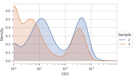
Plot the samples “before”:

>>> flow.Kde1DView(channel = 'CD3',
...                huefacet = 'Sample',
...                scale = 'log').plot(ex)

Create and parameterize the operation.

>>> op = flow.RegistrationOp(channels = ['CD3', 'CD4'],
...                          scale = {'CD3' : 'log',
...                                   'CD4' : 'log'},
...                          by = ['Sample'])

Estimate the clusters

>>> op.estimate(ex)

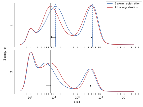
Plot a diagnostic view

>>> op.default_view().plot(ex, plot_name = 'CD3')

Apply the warp

>>> ex2 = op.apply(ex)

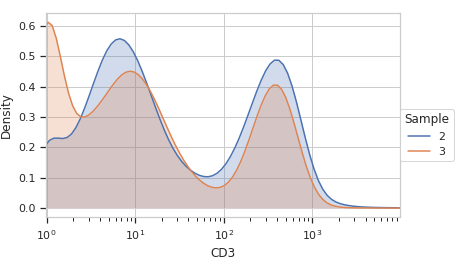
Plot the same KDE after the warp.

>>> flow.Kde1DView(channel = 'CD3',
...                huefacet = 'Sample',
...                scale = 'log').plot(ex2)

estimate(experiment, subset=None)

Estimate the calibration coefficients from the beads file.

Parameters:

experiment (Experiment) – The experiment used to compute the calibration.

apply(experiment)

Applies the bleedthrough correction to an experiment.

Parameters:

experiment (Experiment) – the experiment to which this operation is applied

Returns:

A new experiment with the specified channels warped to bring their density maxima into registration.

Return type:

Experiment

default_view(**kwargs)

Returns a diagnostic plot to see if the peak finding is working.

Returns:

An diagnostic view, call BeadCalibrationDiagnostic.plot to see the diagnostic plots

Return type:

IView

class cytoflow.operations.register.RegistrationDiagnosticView

Bases: HasStrictTraits

A diagnostic view for RegistrationOp.

Plots the smoothed histogram of the bead data; the peak locations; a scatter plot of the raw bead fluorescence values vs the calibrated unit values; and a line plot of the model that was computed. Make sure that the relationship is linear; if it’s not, it likely isn’t a good calibration!

op

The operation instance whose diagnostic we’re plotting. Set automatically if you created the instance using BeadCalibrationOp.default_view.

Type:

Instance(BeadCalibrationOp)

enum_plots(experiment)

Enumerate the named plots we can make from this set of statistics.

Returns:

An iterator across the possible plot names.

Return type:

iterator

plot(experiment, plot_name=None, **kwargs)

Plots the diagnostic view.

Parameters:

• experiment (Experiment) – The experiment used to create the diagnostic plot.

• plot_name (Str) – The channel name to plot.