Tutorial: Hierarchical Gating#
A common strategy for manual gating is hierarchical gating – a skilled cytometrist examines sets of one- or two-dimensional plots, one after another, to separate cells into “positive” and “negative” populations. While I like to think that modern cytometry has better, less biased tools to accomplish this task, it is still a necessary one in many contexts, and Cytoflow supports it.
This tutorial demonstrates a hierarchical gating scheme from Saeys Y, Van Gassen S, Lambrecht BN. Computational flow cytometry: * *helping to make sense of high-dimensional immunology data. Nature Reviews Immunology 16:449-462 (2016). Our question here is a basic one – what is the count of each cell type in each tube in the six tubes in the experiment? The data were downloaded from the Sayes Lab github and compensated using the bleedthrough matrix in the provided FlowJo workspace before being re-saved by Cytoflow – no other data preprocessing was applied.
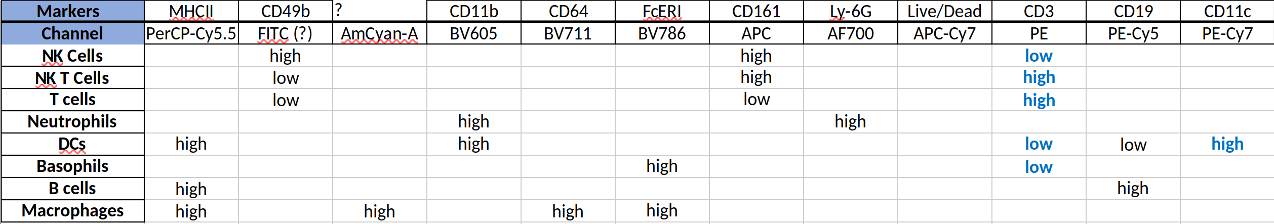
We want to quantify NK, NK T, T and B cells; neutrophils, DCs, basophils, and macrophages. The markers (and the channels they were measured in) are in the table below (also from the Sayes lab github). Per the FlowRepository metadata, these cells were splenocytes from wild-type C57Bl/6 mice.
If you’d like to follow along, you can do so by downloading one of the cytoflow-#####-examples-basic.zip files from the Cytoflow releases page on GitHub.
One final note. I am not an immunologist. This is an explanatory example, using publically available data, to illustrate the software’s functionality. Please don’t write me and tell me I’m using the wrong markers or the wrong dyes.
Import the data#
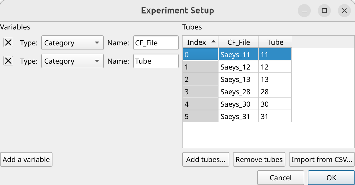
Open the experiment setup panel and set it up as in the image below. We would usually include metadata to make the analysis more biologically meaningful, but I don’t know how (or if) any of these tubes is different.
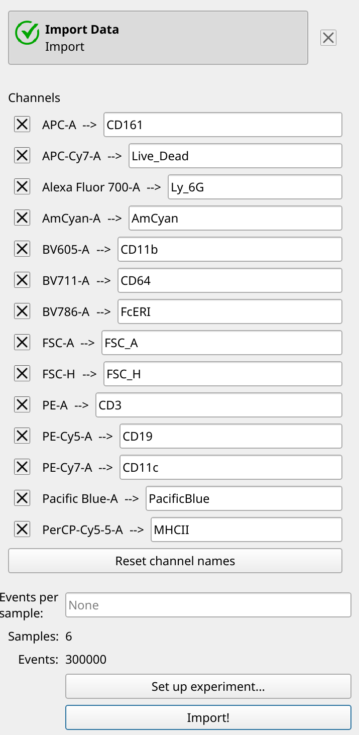
However, we can replace the (uninformative) channel names with the (more informative) markers. (Unfortunately, the metadata on FlowRepository did not say what the AmCyan or Pacific Blue channels were used for, and the FITC channel appears to be unused.)
Gate single cells and live cells#
First, we’ll use a Polygon Gate to select single cells, gating out clumps and debris. Following the gating in the example data, we’ll gate with FSC_A and FSC_H channels on a linear scale. And since there are quite a lot of events in this data set, we’ll use the Density Plot mode (with a log color scale) so we can see what we’re doing.

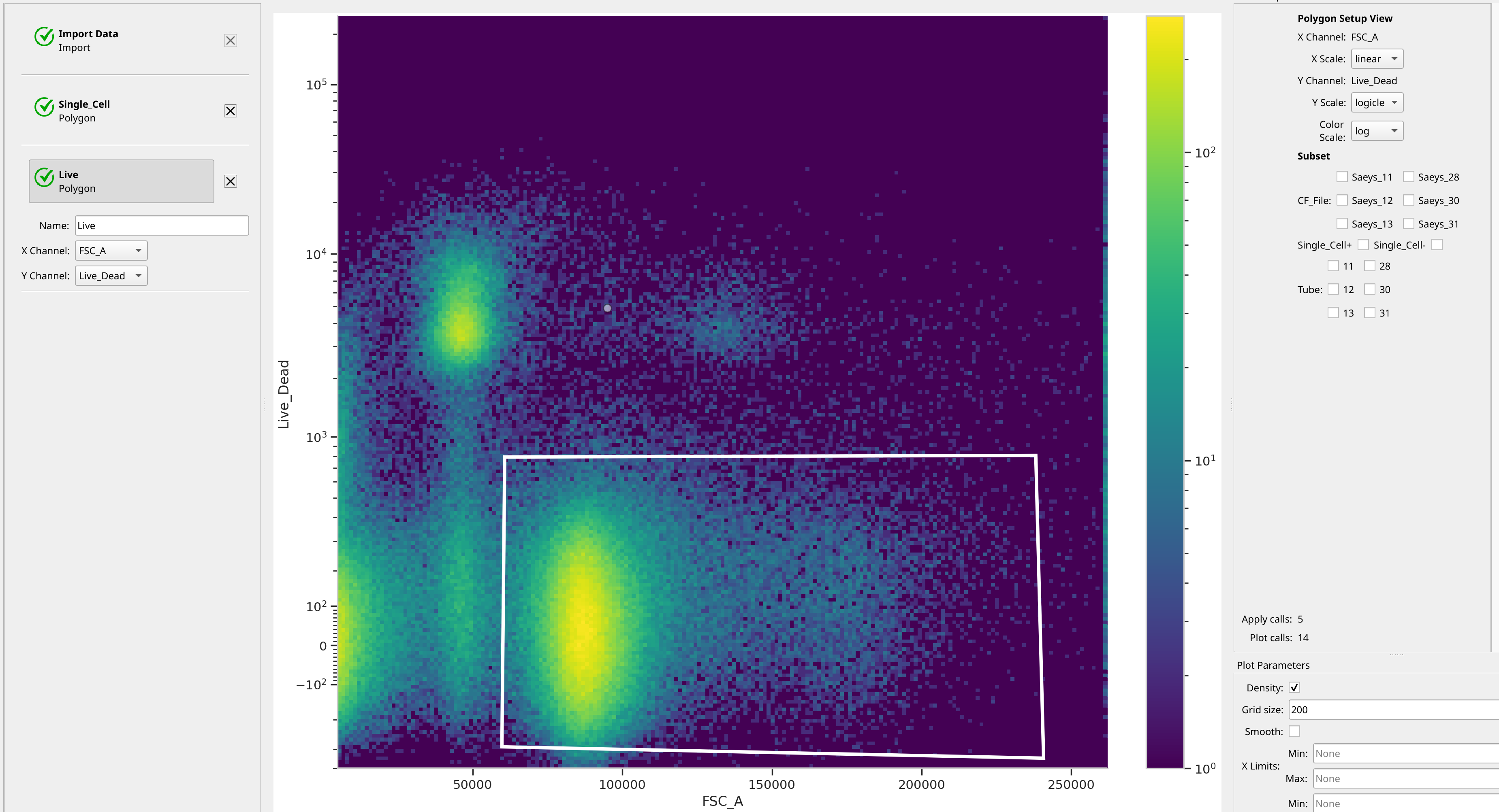
Next, we’ll gate out the live cells with the live-dead marker. The metadata didn’t say which stain was used, but recall that dead cells are positive. We’ll put the linear-scaled FSC_A channel on the X axis and the logicle (biexponential)-scaled Live_Dead channel on the Y axis. Again, we’ll use the Density Plot mode of Polygon Gate to choose the live cells. Increasing the grid size can also make it a little easier to see what we’re doing.
Create Immune Cell Phenotype Gates#
Now, let’s create Polygon Gates for each immune cell phenotype. Note that this is not a strictly hierarchical approach, because each gate I draw will only be on the Single_Cell+ and Live+ plots. The final analysis will be hierarchical, though, as we will see shortly.
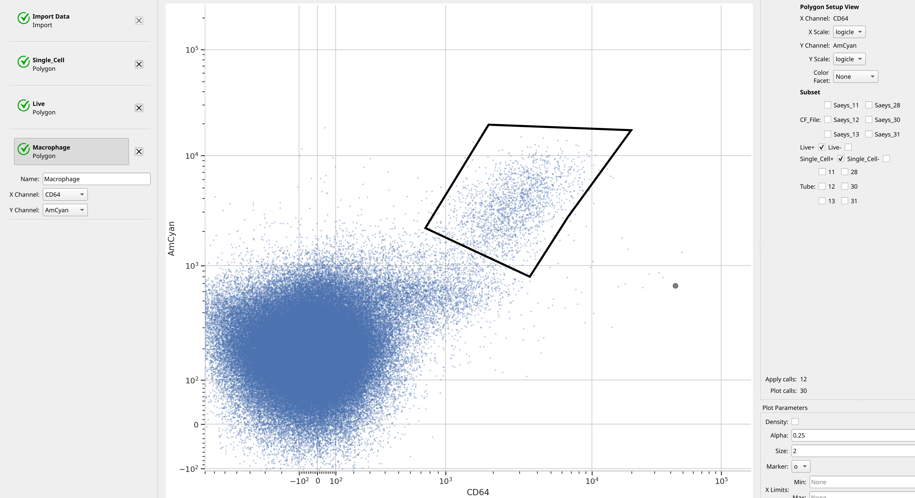
We start with Macrophages, which are CD64+ and AmCyan+. (Remember, I don’t know what marker is being measured in the AmCyan channel….)
B cells are CD19+ and CD3-.

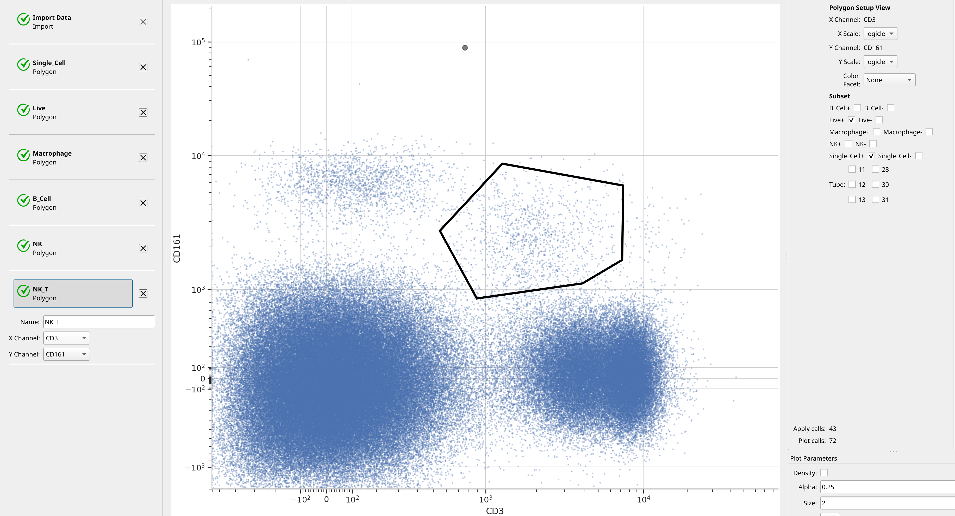
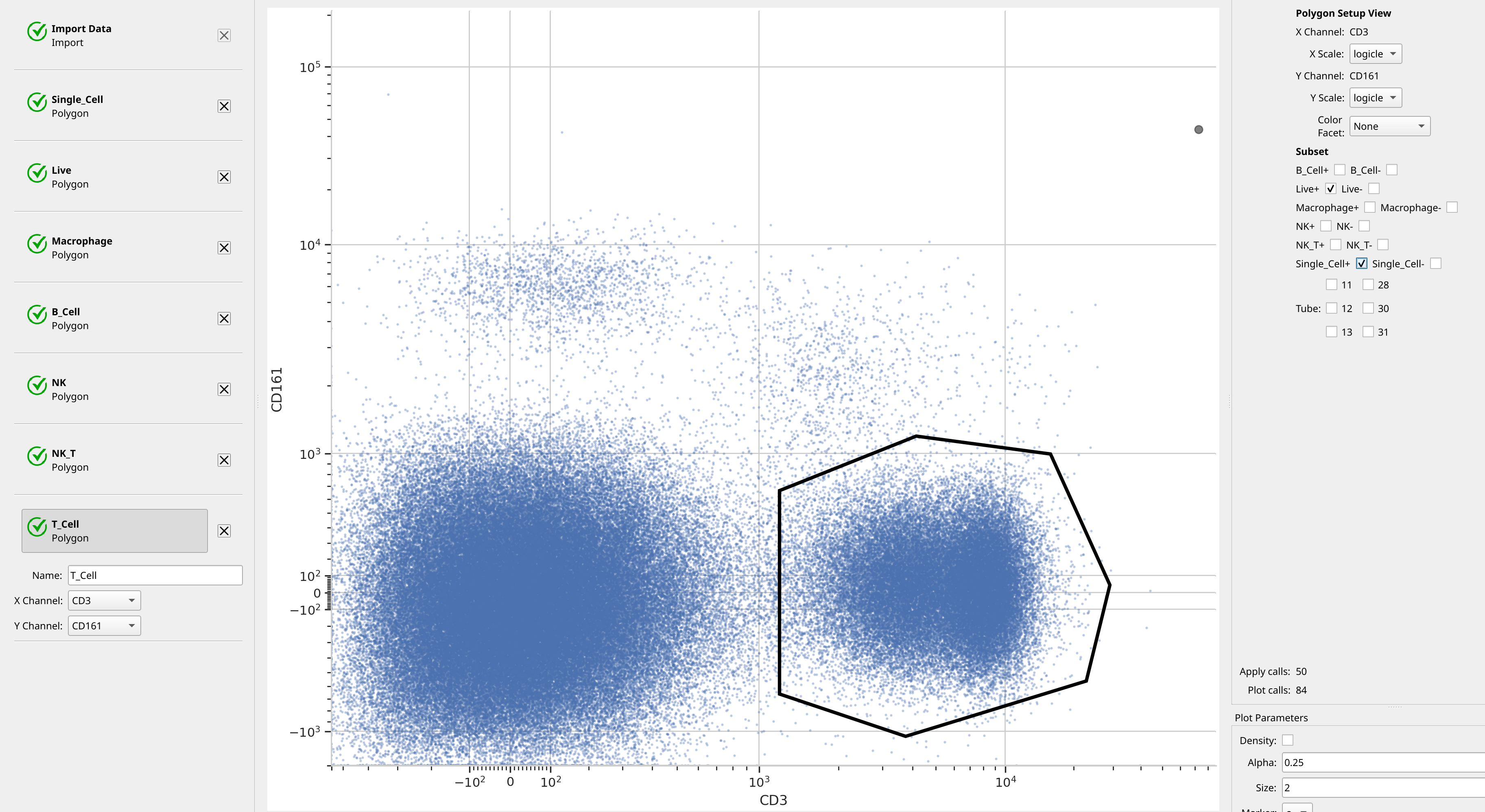
CD3 and CD161 can distinguish NK, NK T and T Cells.

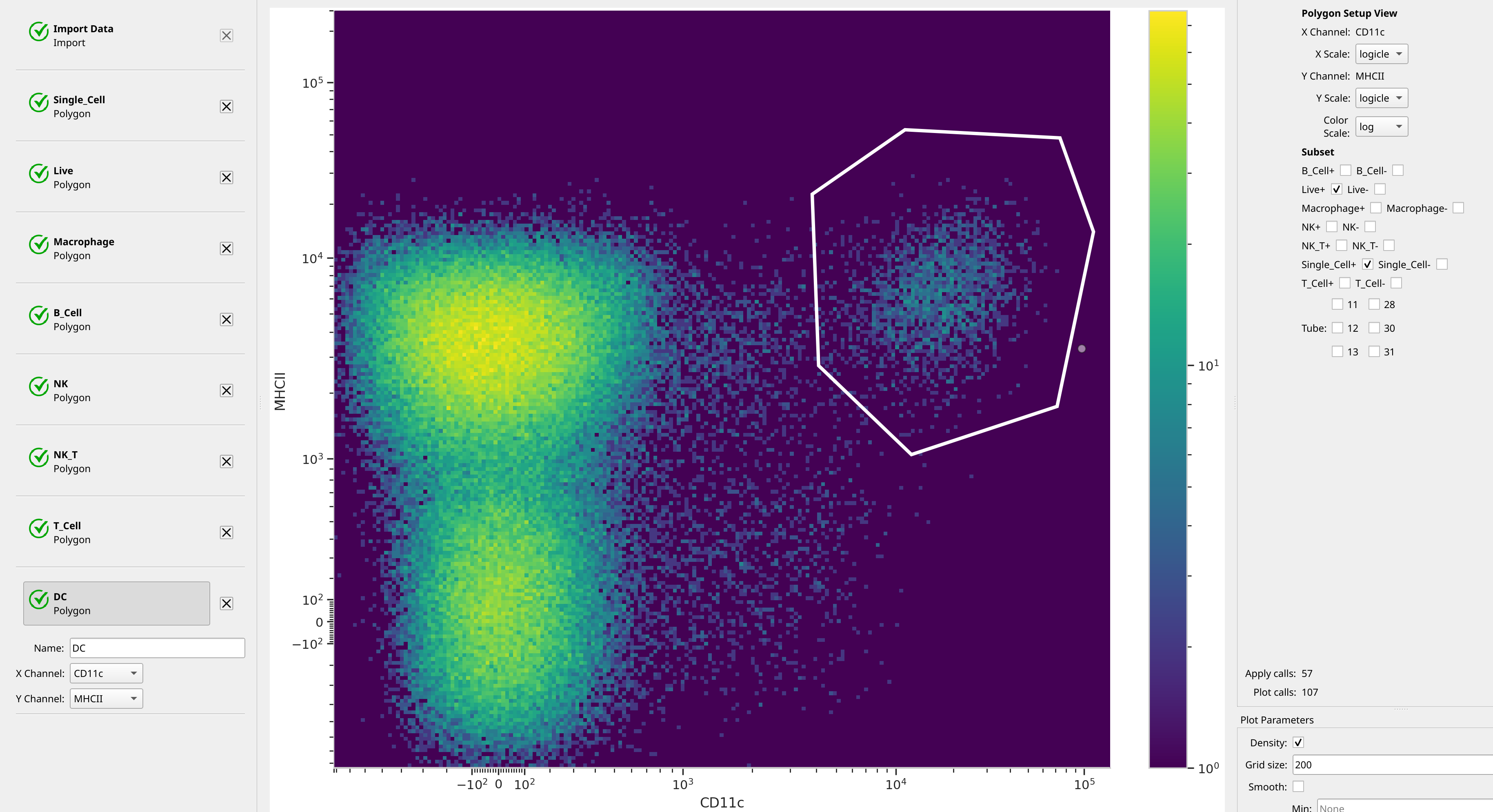
Almost done. DCs are CD11c+ and MHCII+. And let’s use a density plot, for giggles.
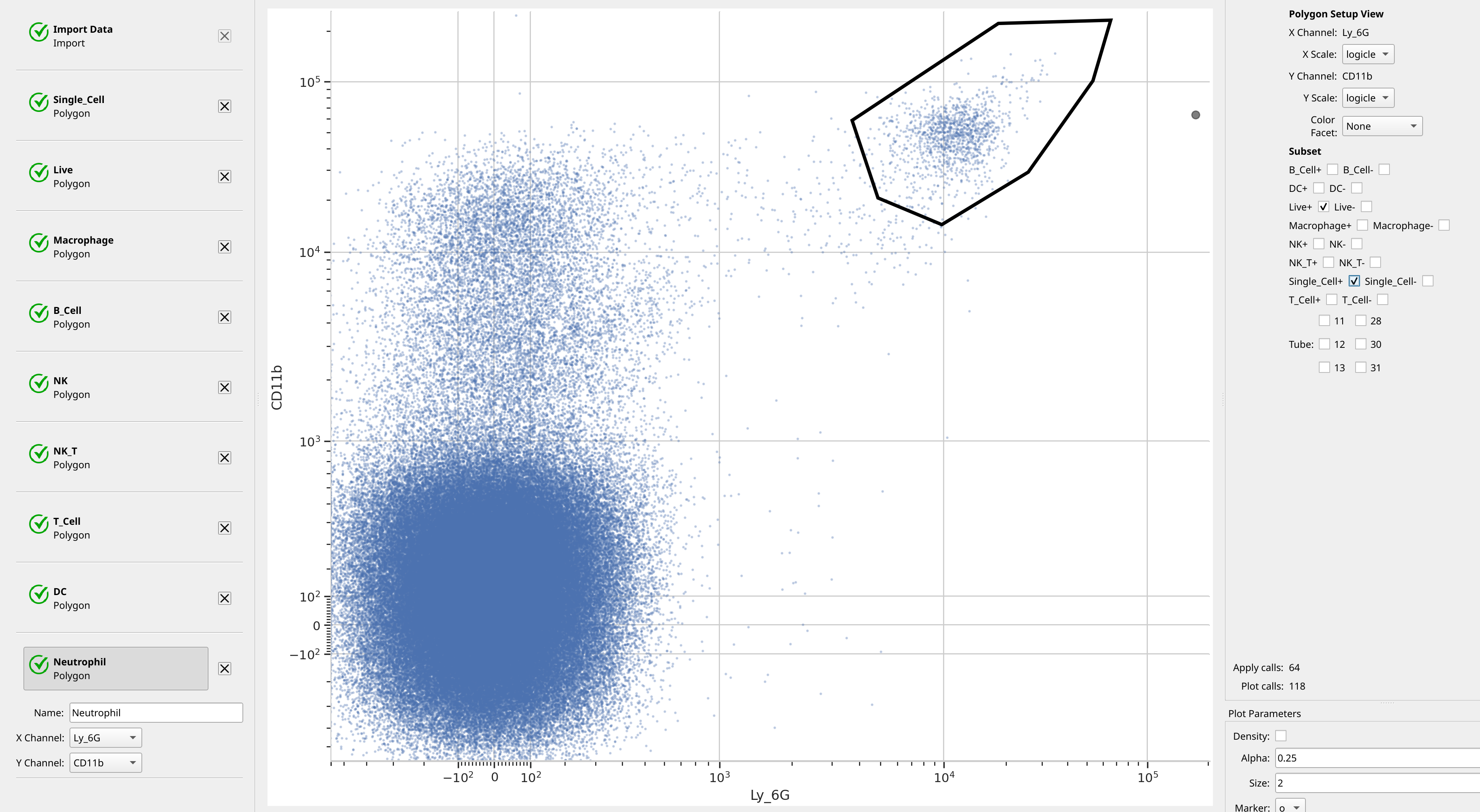
Neutrophils are Ly_6G+ and CD11b+.
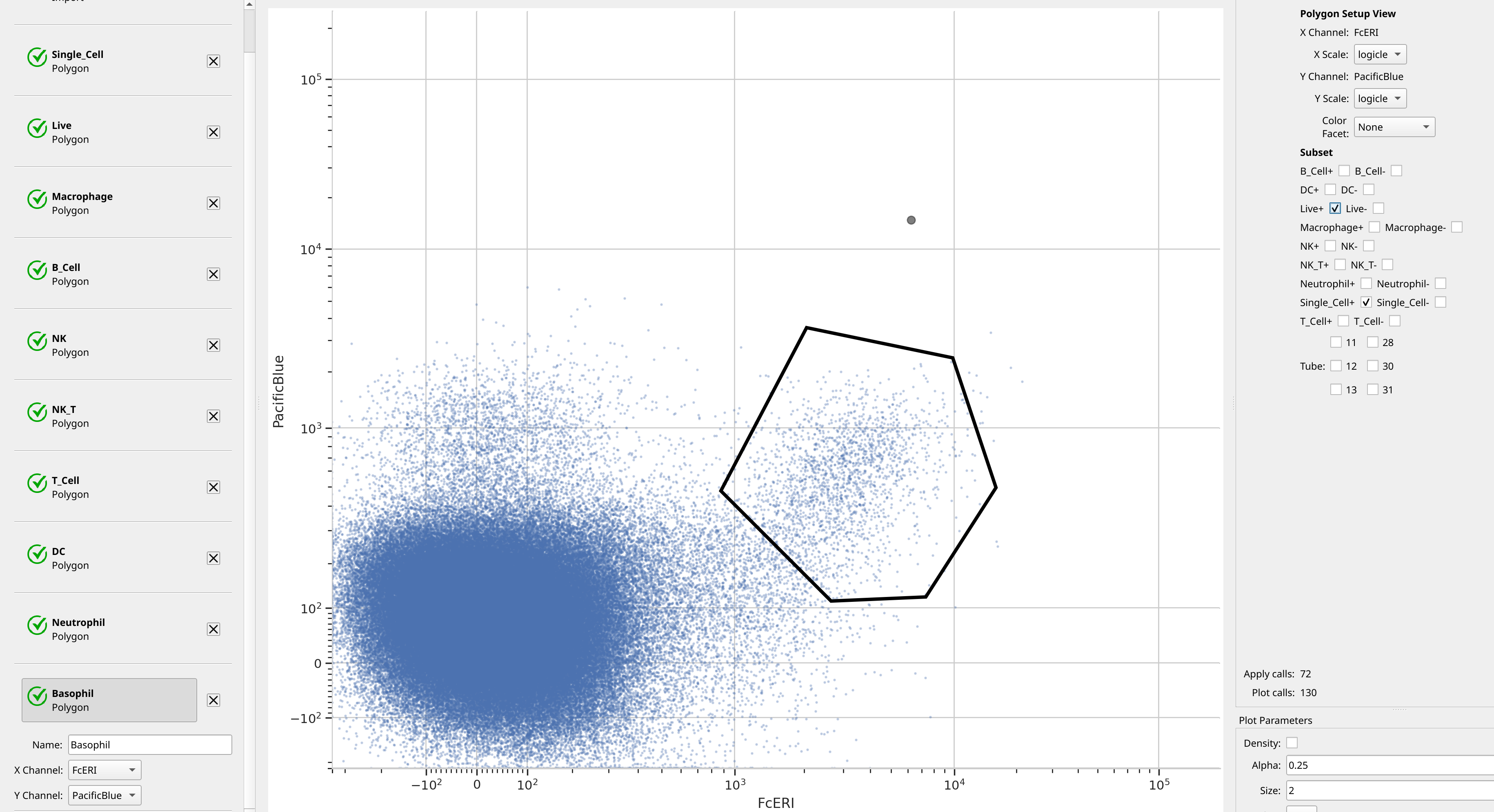
And finally, Basophils are FcERI+ and Pacific Blue+. (Again, I don’t know what marker is on the Pacific Blue channel.)
Analyze the hierarchy#
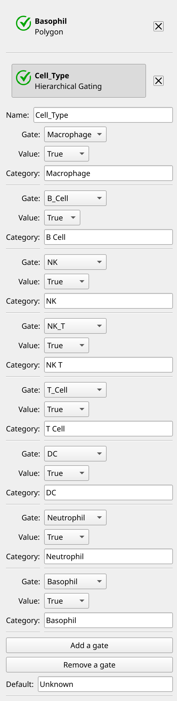
The way Cytoflow allows you to analyze a hierarchical gating scheme is by creating a new condition using the Gate Hierarchy operation. As we will see, you specify an ordered list of gates, the values of those gates, and the labels you’d like to assign to events in each gate. A label in the new condition is assigned for each event in the following manner:
Membership in the first gate is evaluated. If the event’s value is the same as the one specified, it gets the first label.
If not, then membership in the second gate is evaluated. If the event’s value is the same as the one specified, it gets the second label.
This process continues until we’re out of gates. In this case, the event’s label is assigned some default value, often “Unknown”.
So, set up the Gate Hierarchy operation as below:
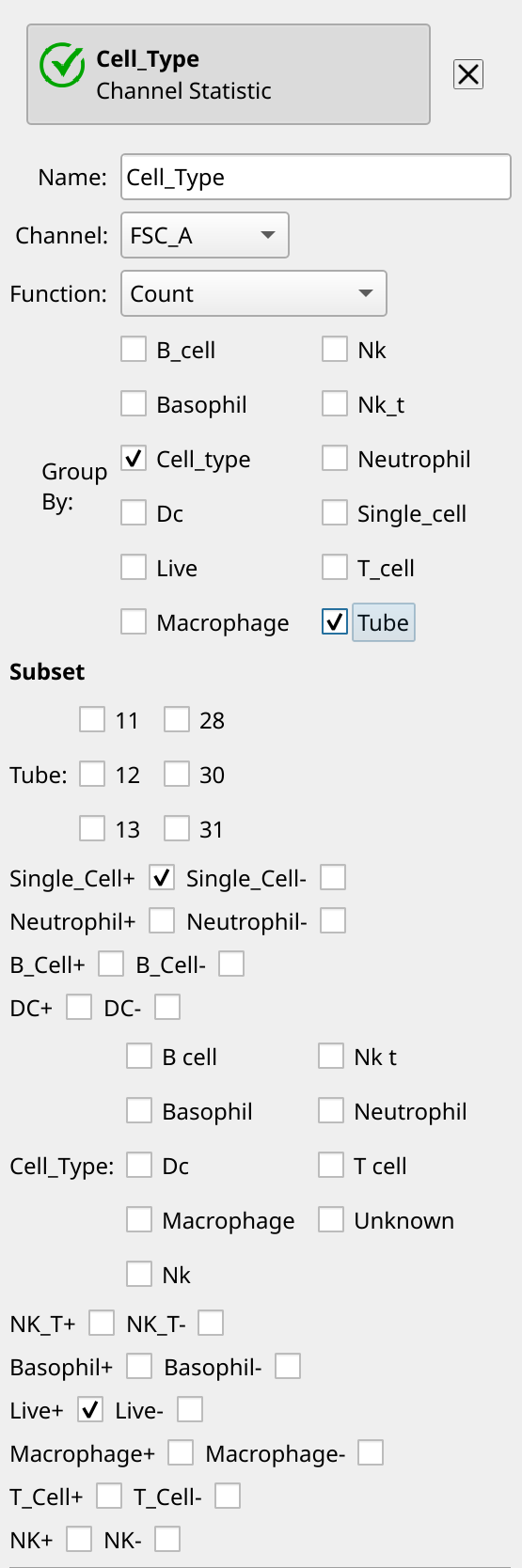
Now we’ve got a new condition called Cell_Type that implements our hierarchy, and we can compute statistics as usual. For example, we can count the cells in each category in each tube with a Channel Statistic operation. Note how we’re grouping by both Cell_Type and Tube, and only counting Live and Single_Cell cells.
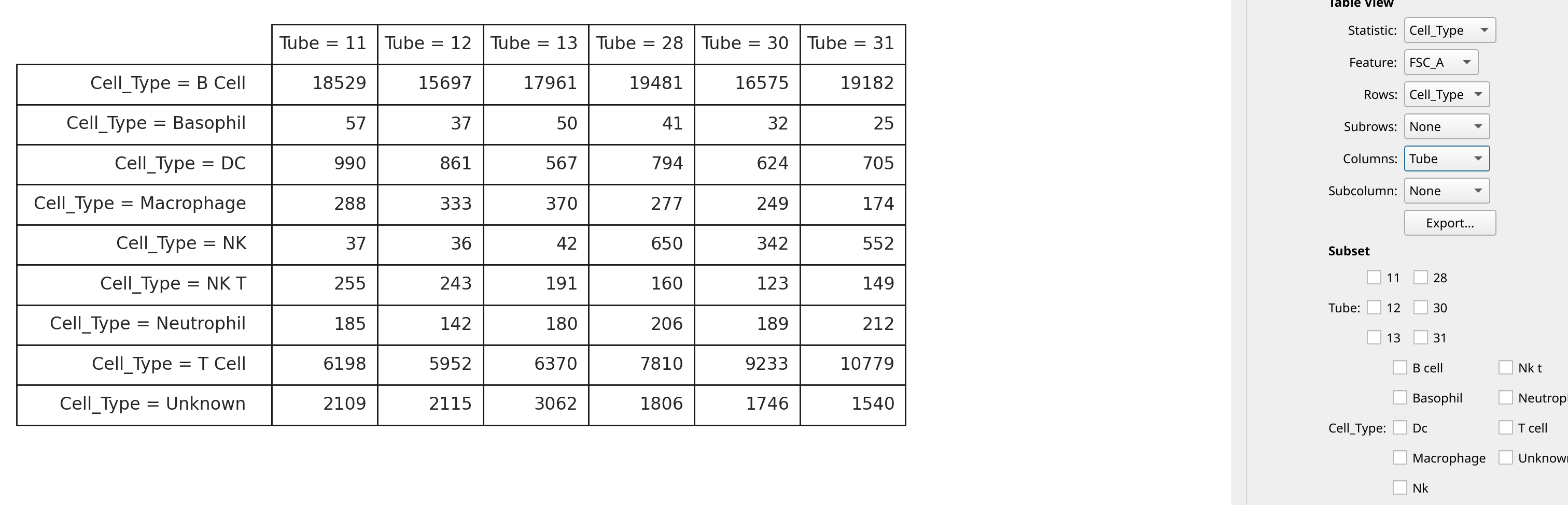
We can look at the new statistic as a table:
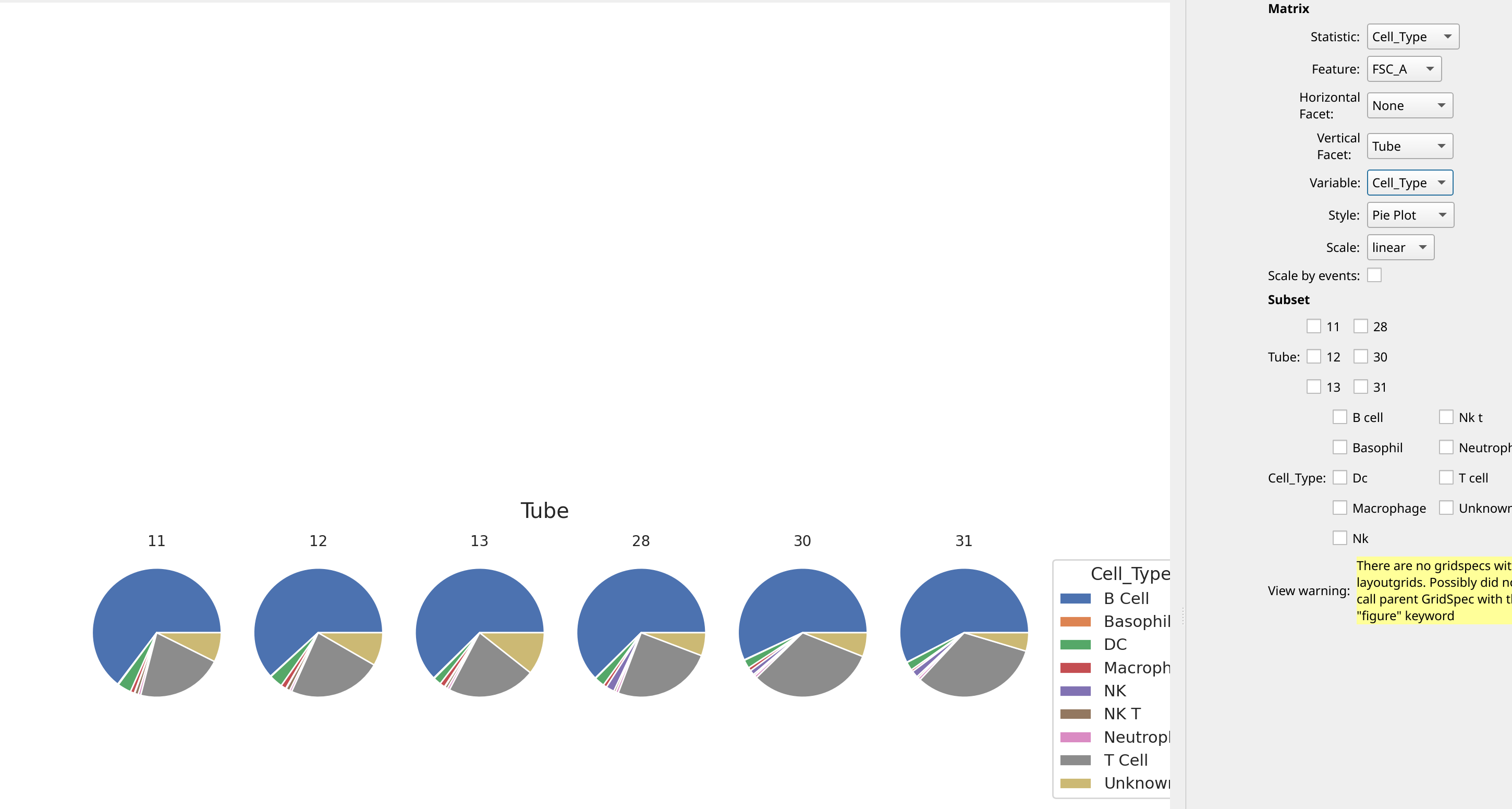
We can also make pie plots using the Matrix view: