Tutorial: Estimating Genome Size

Flow cytometry is regularly used to estimate genome size relative to a standard, often in plants. Nuclei are isolated from a plant of unknown genome size and from a plant of known genome size; the samples are mixed, stained with a fluorescent DNA-binding dye such as DAPI, and run on a flow cytometer. The relative fluorescences can be used to estimate the size of the unknown genome relative to the known one.

This tutorial demonstrates one possible approach. We use data from Kúr et al. Cryptic invasion suggested by a cytogeographic analysis of the halophytic Puccinellia distans complex (Poaceae) in Central Europe. Frontiers in Plant Science 14, 2023 DOI: 10.3389/fpls.2023.1249292. No pre-processing was done – these are the raw files downloaded from the publication’s dataset on Zenodo. I did remove one file whose data looked pretty wonky – the investigators do the same with several of their samples.

If you’d like to follow along, you can do so by downloading one of the cytoflow-#####-examples-basic.zip files from the Cytoflow releases page on GitHub. These data are in the data/genome_size subfolder.

Import the data

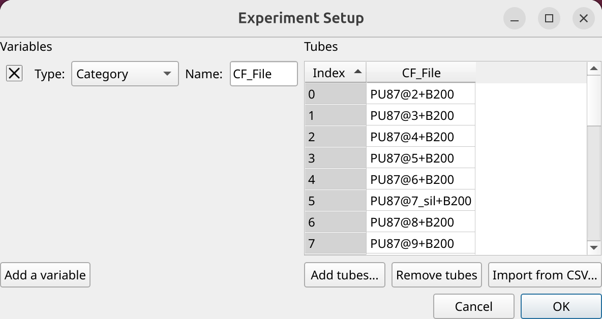
Open the experiment setup panel and select all of the files. (Remember, you can click the first, then shift-click the last, to select multiple files.) Because we don’t have any metadata besides the filename, change the CF_File column type to Category and click OK.

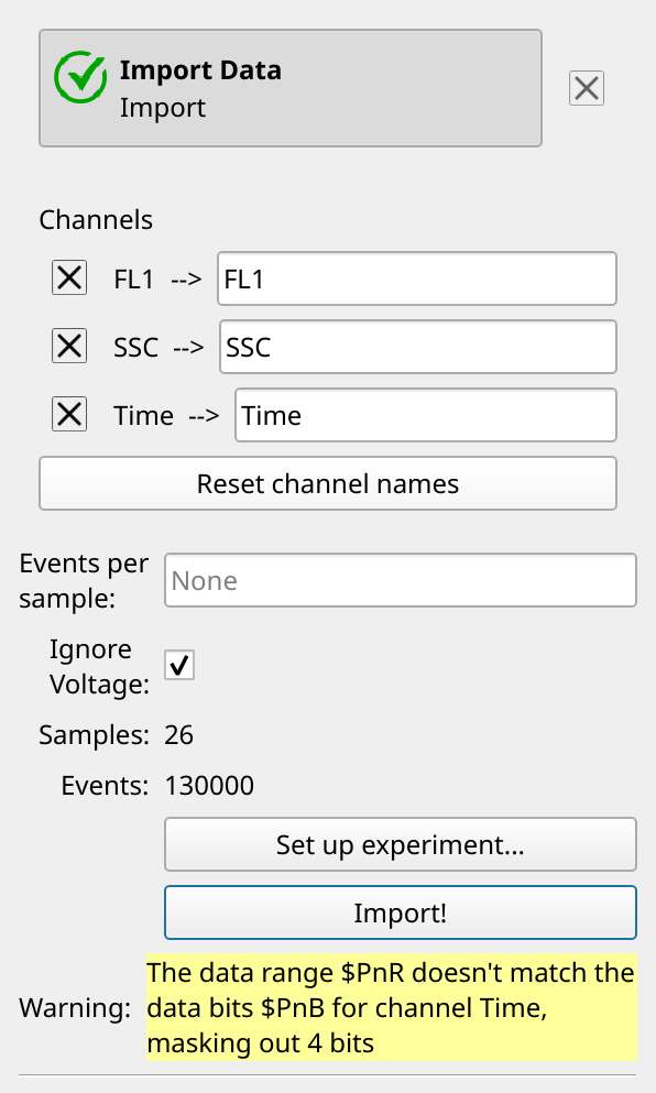
Usually Cytoflow imposes a constraint that a channel’s voltages are the same for each FCS file it imports. With care, this can allow you to compare quantitative measurements across FCS files. However, occasionally you need to relax this constraint, and this is one of those times – a few of these FCS files have slightly different voltages. However, because the standard is spiked into each sample, we can safely proceed. So, enable Ignore Voltages and click Import.

Note

You can safely ignore the warning. Occasionally an instrument manufacturer’s software saves files a little strangely. Cytoflow knows about a lot of these issues and fixes them for you, but it will also warn you that the data it is analyzing is not exactly the data in the FCS files.

Take a look at the data

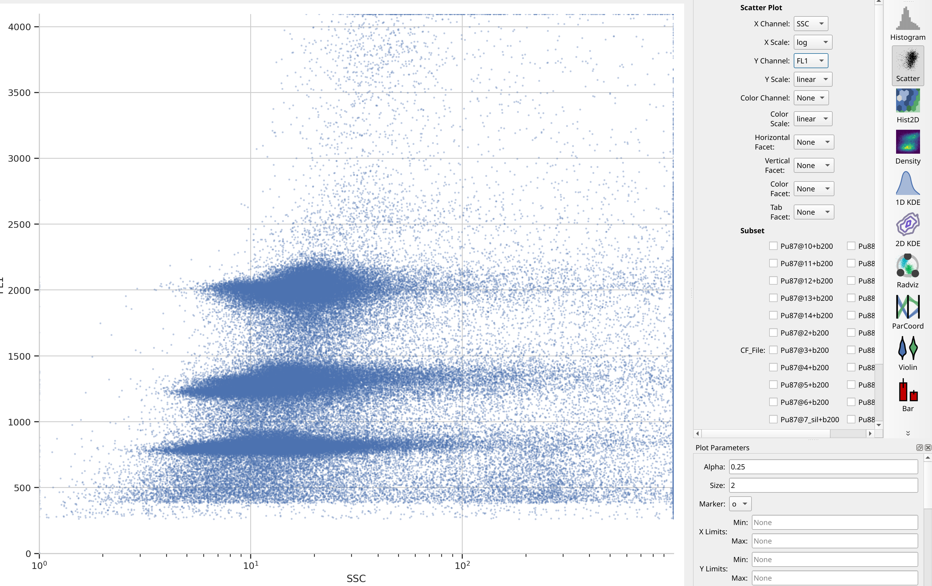
It’s always good to start with some basic data exploration. Here, there are only two channels saved (in addition to Time), so have a look at the scatter plot. Notice that there are three major clusters – the lower FL1 cluster is our internal standard, and the higher two clusters are the nulcei we’re trying to estimate. There’s also quite a bit of noise, which might make that estimation inaccurate – we’ll think about that in a minute.

Tip

Remember that unless you facet or subset your plot – which we’re not doing here – you’re looking at the whole data set, all of the tubes together on one plot.

Gate out the high SSC events

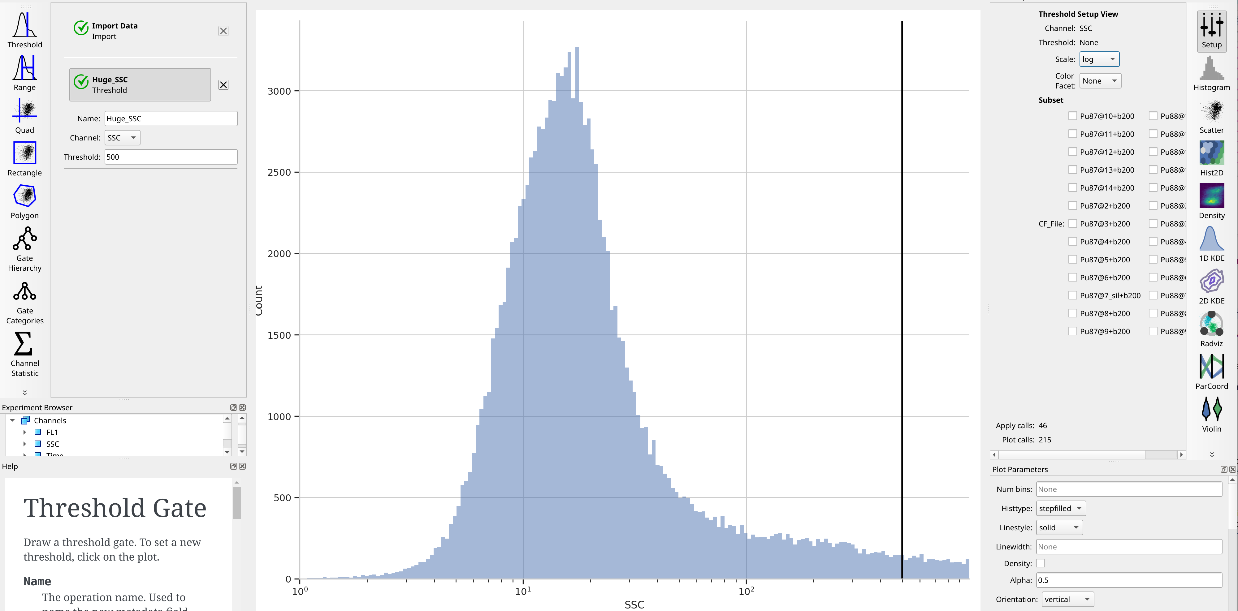
Let’s at least get rid of the saturating events on the SSC channel. To do so, create a Threshold gate, name it Huge_SSC, set the channel to SSC and set the threshold to 500.

Find the peaks with a density gate

Let’s assume, for the minute, that we don’t want to draw 40 different gates to find the two peaks in each of our 20 samples. What to do? Cytoflow includes several automated clustering algorithms, and the one that works best in this situation is a Density Gate. The user selects how much of the data they would like to retain, and this gate selects that proportion of events in the highest-density regions of a 2D plot. Most important for our use, we don’t have to use the same gate for the entire data set. Like most data-driven operations, the Density Gate lets you group the data by some condition or piece of metadata before estimating the operation’s parameters. In this case, we’ll compute a different gate for each tube.

Let’s keep 45% of the data – you’ll see why in a moment. Name the gate Density and gate on the SSC and FL1 channels, same as the scatterplot. Change the X Scale from log to logicle, though. To make a different gate for each tube, set Group Estimates By to Cf_file. And make sure you choose Huge_SSC- under Subset to ignore the events with huge SSCs.

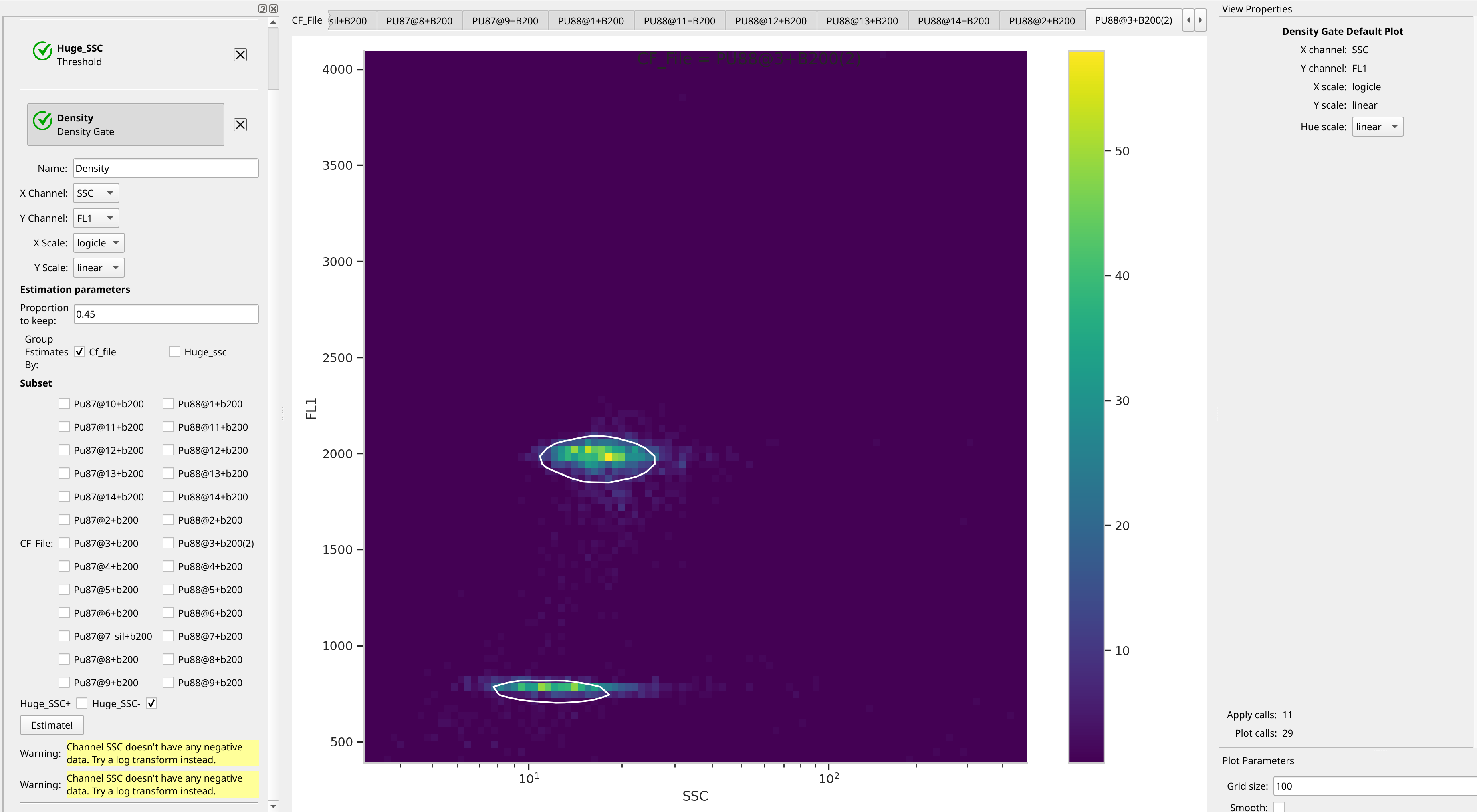
Glance through the plots and see what the Density Gate operation has done: it has found the peaks for each tube! Even when those peaks moved! And now we can see why I used 45% – this was a value that found both peaks in all of the tubes.

Note

While a data-driven operation such as Density Gate can estimate different model parameters for each subset – as it did here, a different gate for each tube – the operation parameters must be the same for each subset. For example, you can’t keep 45% of the events for one tube and 60% for another.

Note

Why change the X scale? This was another issue I caught as I scrolled through the gates – there was a gate with strange behavior with events with very small SSCs. I could have gated them out, I suppose, or I could change the scale – logicle behaves much better around 0 than log does.

Separate the control and the sample peak

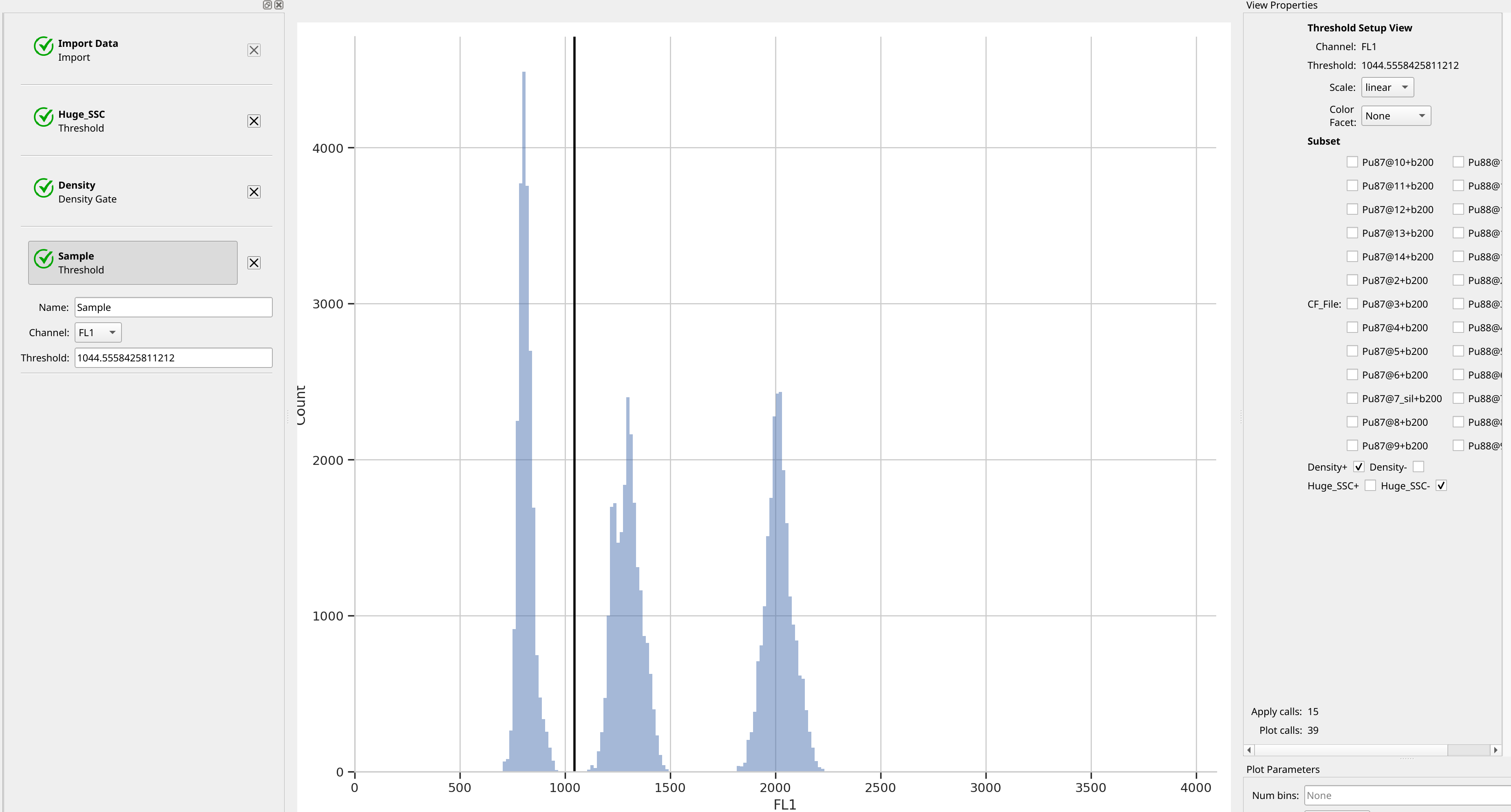
We’ve found the peaks, but if we want to summarize the different peaks’ means separately, we need to separate them. Let’s do so with another threshold gate – this one I’ll name Sample, to distinguish the sample from the control.

Note that in the setup view, I’ve selected Density- – this hides all the events that weren’t in the peaks and cleans up the plot substantially.

Compute the peaks’ means

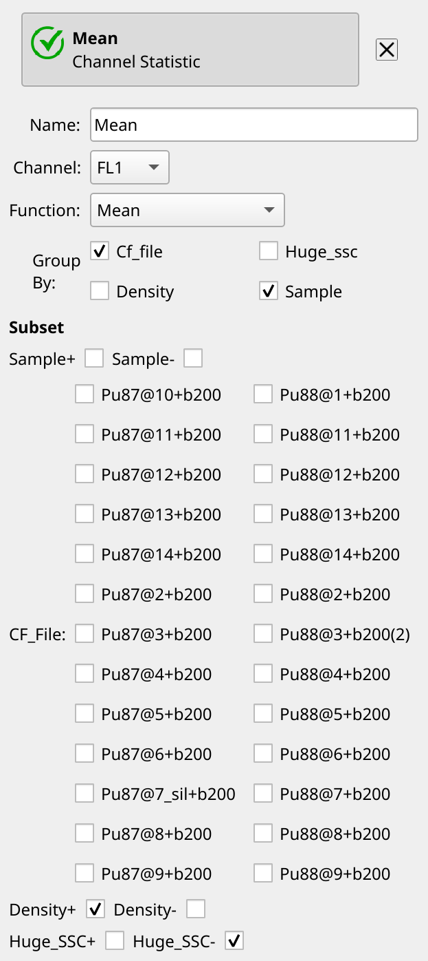
We’re almost done. Recall that in Cytoflow, if we want to summarize some flow data, we do so by creating a statistic. So let’s create one using the Channel Statistic operation. Name it Mean, set the channel we’re summarizing to FL1, and the function to Mean. Group by both Cf_file and Sample – we want both peaks’ means – and set the subset to Density+ and Huge_SSC-. There’s no Estimate! button – the operation updates each time you change a setting.

Finally, we can view our statistic using the Table view. Each of the conditions we grouped the statistic computation by becomes a “variable” (technically, a facet) in the new statistic, and we can assign each to the rows or columns (or subrows or subcolumns) in the table. In this case, let’s put each file on a row and each value of Sample on a column.

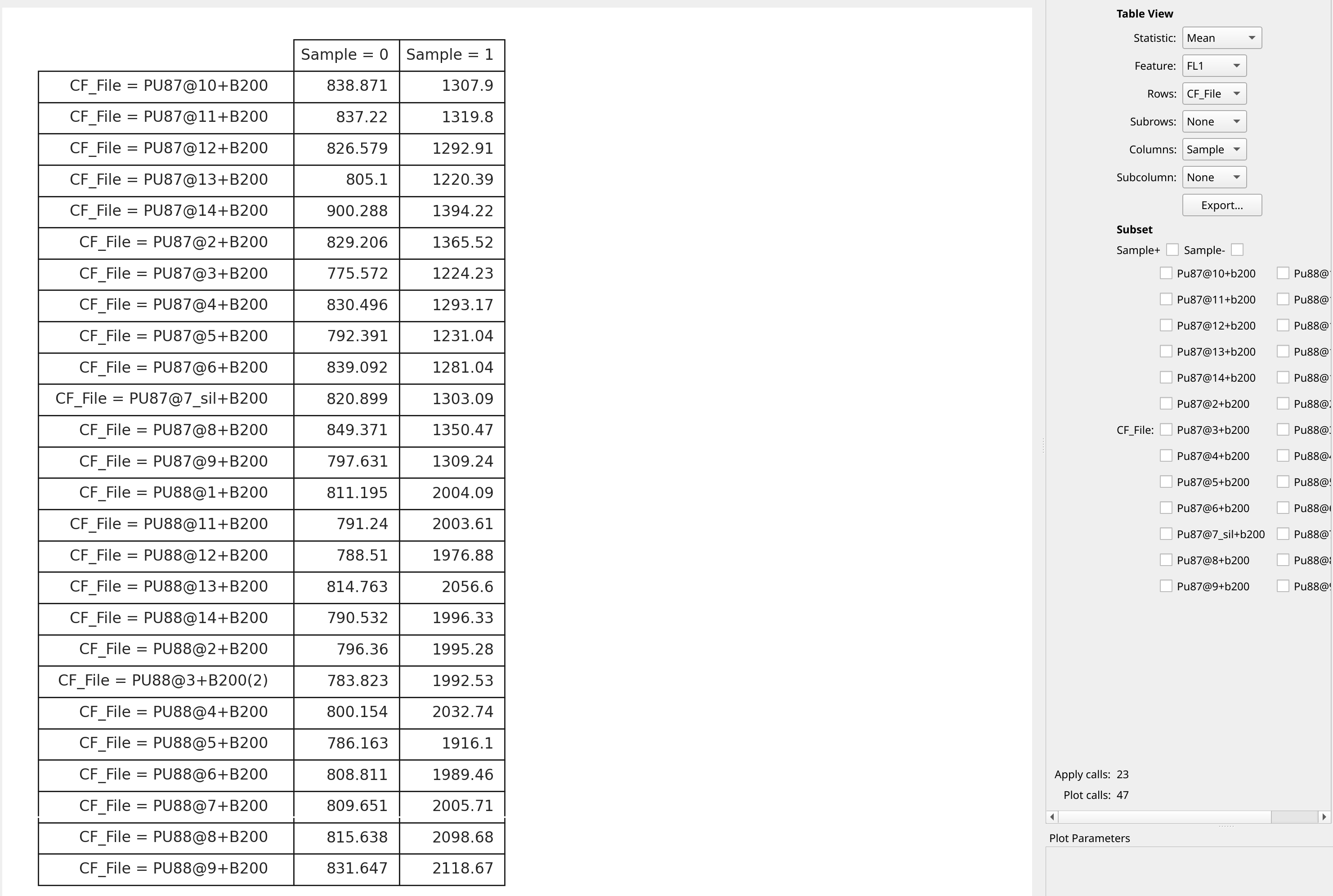
Recall that Sample = 0 are the internal control peaks, and Sample = 1 are the unknown peaks. A little more math in a spreadsheet program will find the ratio between the two and convert to pg DNA per nucleus.

Tip

Remember, you can export this table to a CSV file with the Export button!