HOWTO: Use the TASBE workflow for calibrated flow cytometry

As outlined in HOWTO: Use beads to correct for day-to-day variation, flow cytometry’s quantitative power is somewhat belied by the sensitivity of single-cell measurements to instrument configuration and state. In a word, cytometers drift – sometimes by as much as 20% over the course of a day, even with identical settings. This can complicate experiments or processes that depend on precise, reproducible measurements – predictive modeling of gene expression in particular.

Fortunately, a set of data manipulations can go a long way towards fixing these issues:

• Subtract autofluorescence from the experimental measurements. This requires the measurement of a non-fluorescent control.

• Compensate for spectral bleed-through. This requires the measurement of controls stained with (or expressing) the individual fluorophores alone.

• Calibrate the measurements using a stable calibrant. This requires measuring a calibrant such as the Spherotech rainbow calibration particles

• (Optional) Translate all the channels so they’re in the same units. This requires the measurement of multi-color controls where the staining (or expression) of each fluorophore is equal.

You can read more about this workflow in the following resources:

• A Method for Fast, High-Precision Characterization of Synthetic Biology Devices

• Accurate Predictions of Genetic Circuit Behavior from Part Characterization and Modular Composition

• The TASBE Jupyter notebook

Because this method originated in software called Tool-Chain to Accelrate Synthetic Biology Engineering, we abbreviate it TASBE. And while it was developed in the context of modeling and simulating synthetic gene networks, there is nothing about it that is syn-bio specific. If you want to generate data sets that you can directly compare to eachother (particularly if they’re collected on the same instrument), this is the calibration that will let you to so. And while each of the steps above has its own operation, they’re also combined in the TASBE operation.

Procedure

1. Collect the following controls:

   • Blank, un-stained, non-fluorescent cells (to subtract autofluorescence).

   • Cells stained with (or expressing) only one fluorophore (to compensate for spectral bleedthrough).

   • Beads (to calibrate the measurements)

   • (Optional) multi-color controls, where each pair of fluorescent molecules stains (or is expressed) at equal intensity.

2. #. Import your data into Cytoflow. Do not import your control samples (unless they’re part of the experiment.) In the example below, we’ll have three fluorescence channels – Pacific Blue-A, FITC-A and PE-Tx-Red-YG-A – in addition to the forward and side-scatter channels.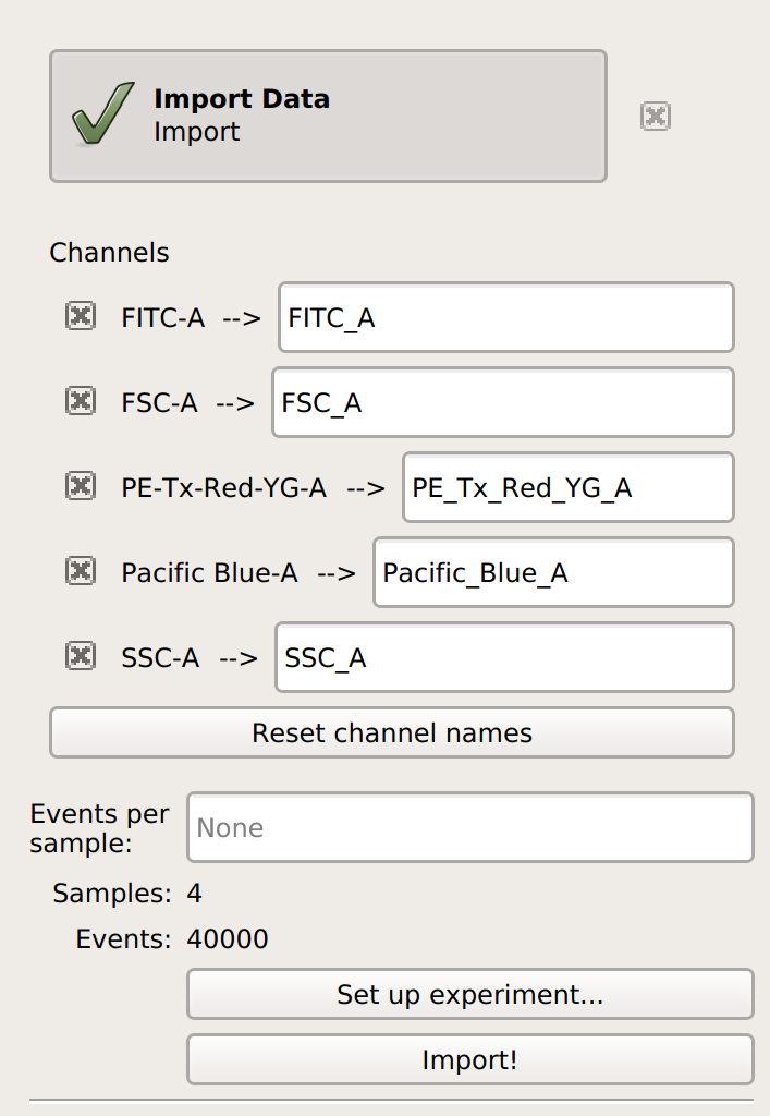

   

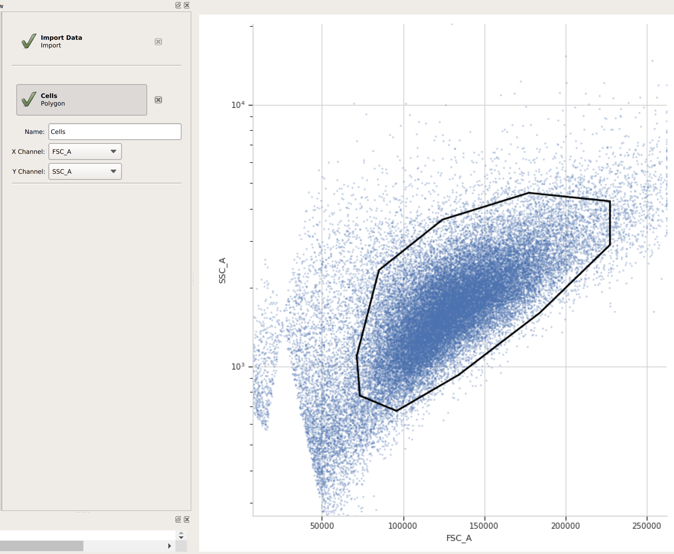
3. (Optional but recommended) - use a gate to filter out the “real” cells from debris and clumps. Here, I’m using a polygon gate on the foward-scatter and side-scatter channels to select the population of “real” cells. (I’ve named the population “Cells” – that’s how we’ll refer to it subsequently.

   

4. Add the TASBE operation (it’s the button).

   

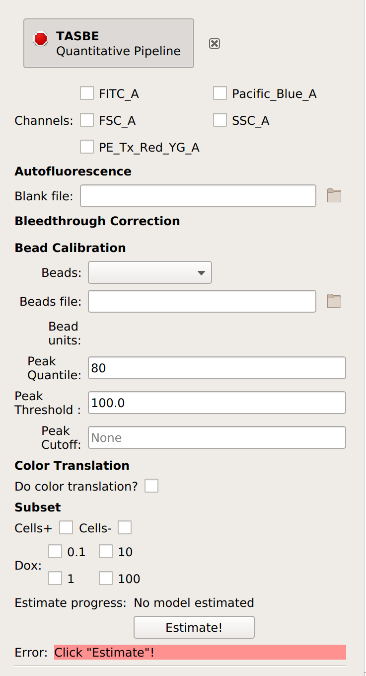
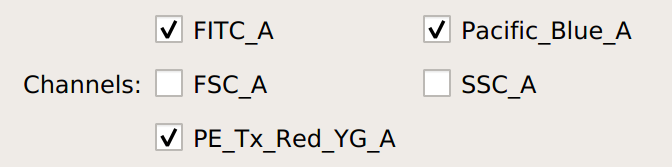
5. Select which channels you are calibrating.

   

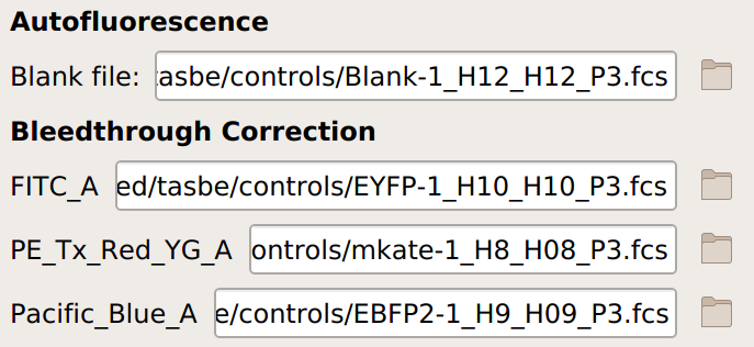
6. Specify the files containing the blank and single-fluorophore controls.

   

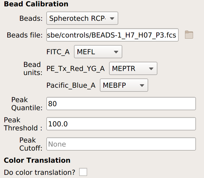
7. If you are not doing a unit translation: select the beads you’re using, the data file, and the appropriate units for each channel:

   

8. If you are doing a unit translation, specify the beads you’re using, the data file, the unit you want all the channels in, the channel you want everything translated to, and the multi-color control files.

   

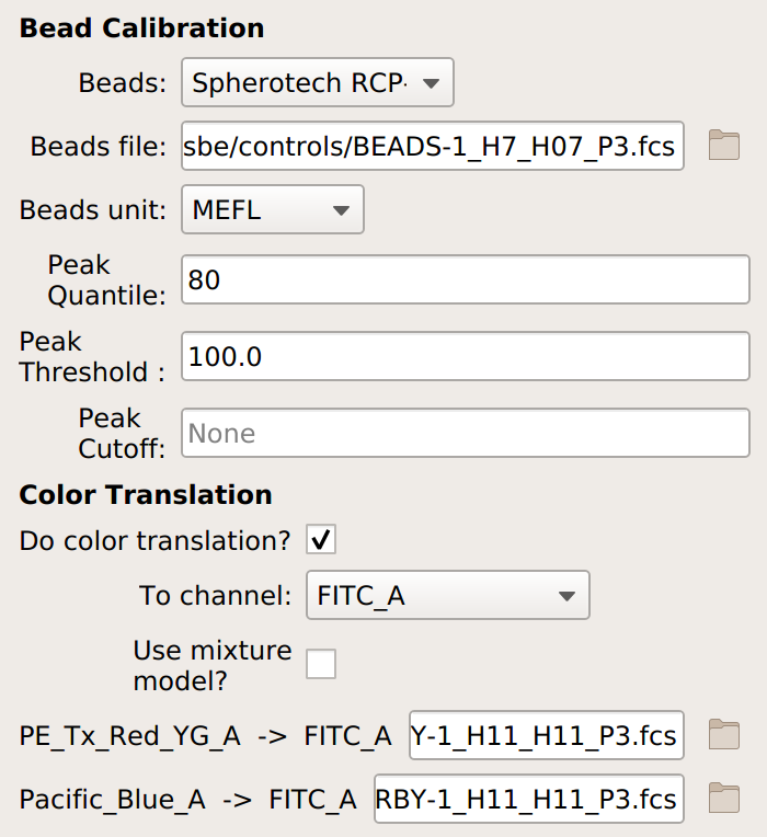
   Note

   If you’re measuring cells that have a large non-fluorescent population – such as transfected mammalian cells – choose Use mixture model as well.

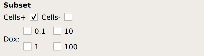
9. (Optional but recommended) - if you set a gate above to select for cells (and not clumps or debris), select that gate under Subset:’

   

10. Click Estimate!

11. Check all three (or four) diagnostic plots – make sure that the estimates look reasonable.

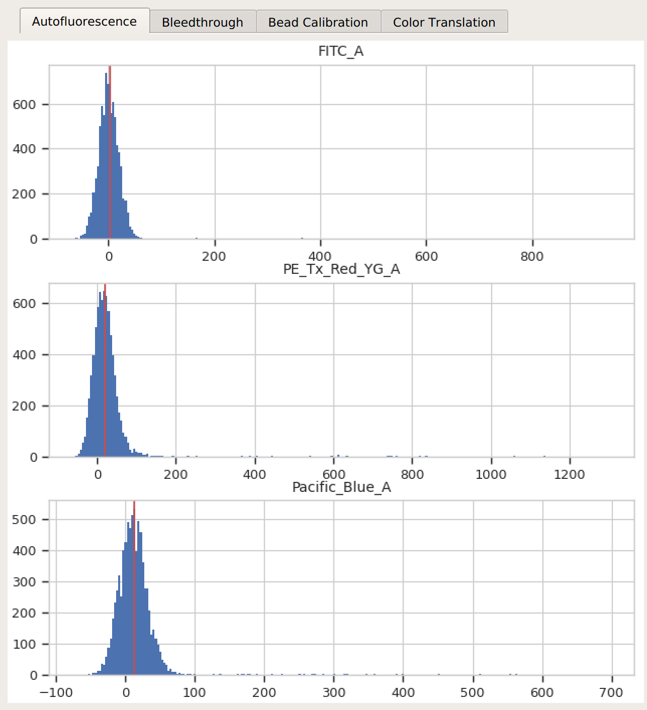
    • Autofluorescence – there’s a single peak in each channel, and a red line at the center.

      

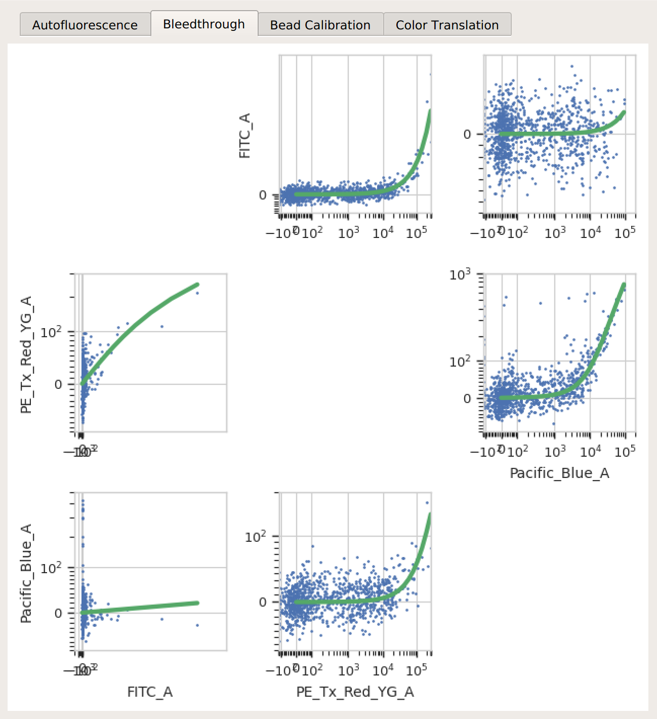
    • Bleedthrough – the bleedthrough estimates (green lines) follow the data closely.

      

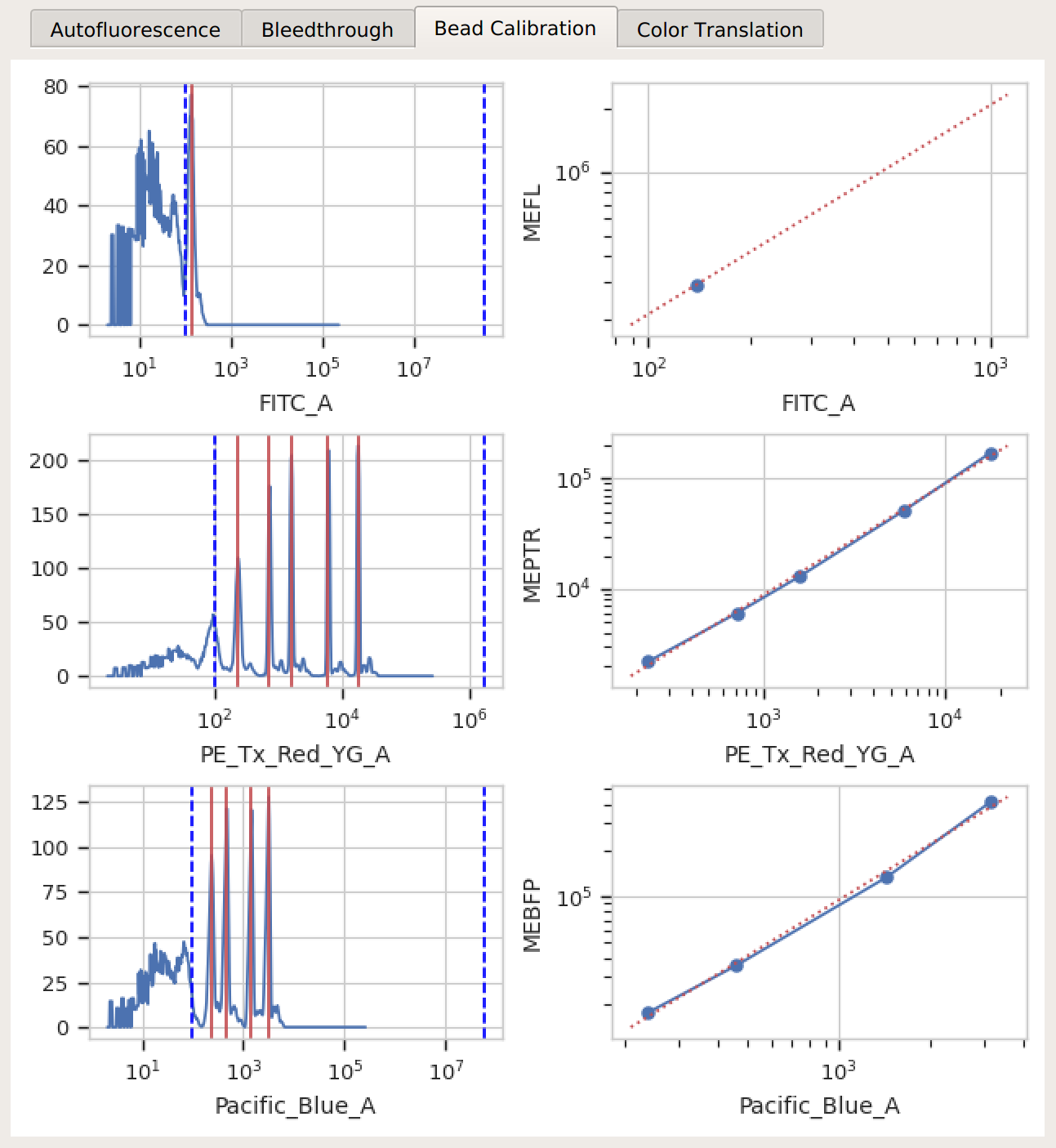
    • Bead Calibration – all the peaks between the minimum and maximum cutoffs (blue dashed lines) were found, and there’s a linear relationship with the vendor-supplied values.

      

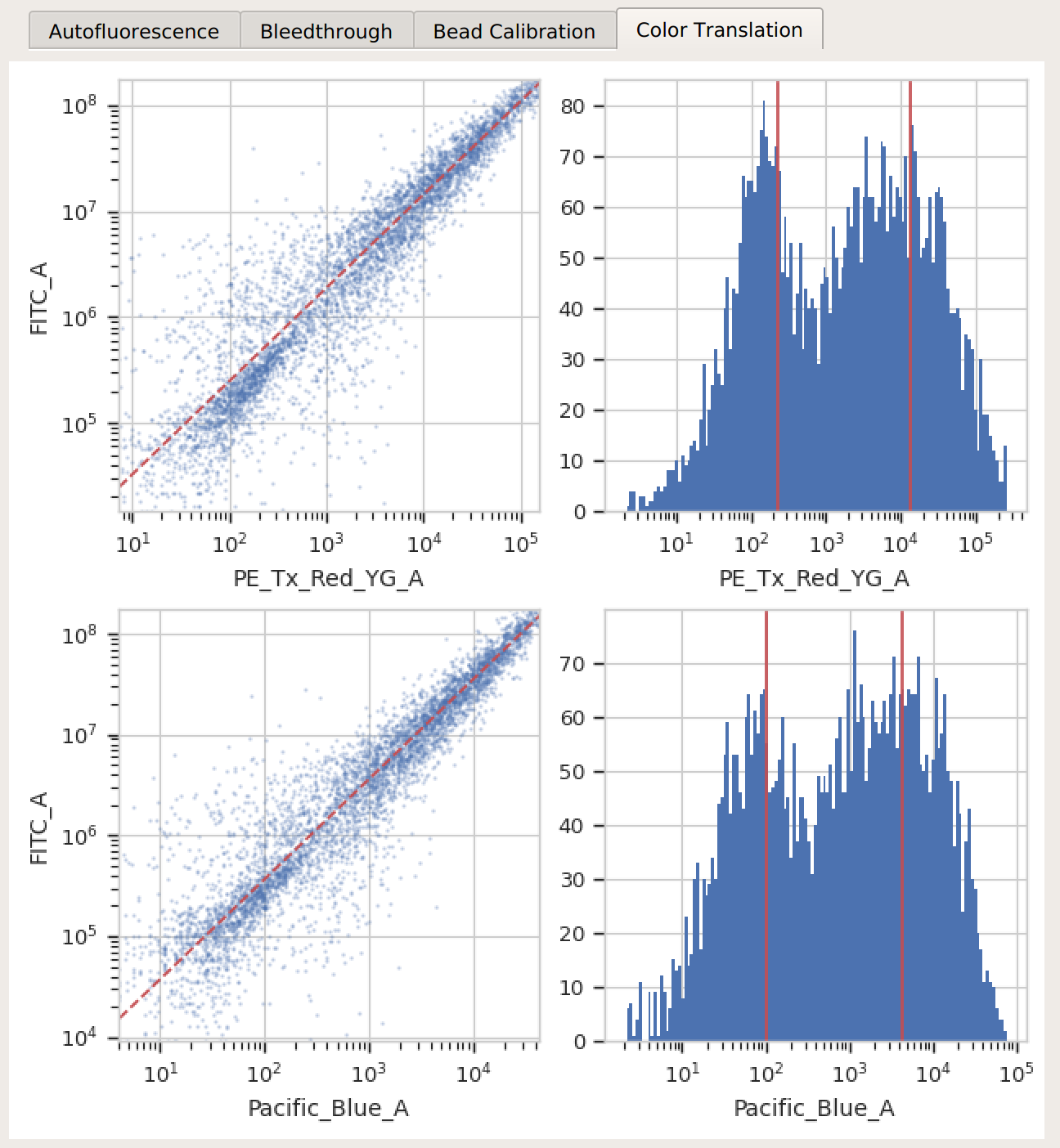
    • Color translation – there’s a linear relationship between the channels, and if you’re using a mixture model, the centers of the two distributions were successfully identified.

      

12. Proceed with your analysis. If this will involve multiple data sets from multiple days, you may wish to export the calibrated data back into FCS files, as described here: HOWTO: Export FCS files.