HOWTO: Compensate for bleedthrough

One common issue in flow cytometry is the fact that spectrally adjacent channels often overlap. For example, if I’m trying to measure a green fluorophore like FITC, and a yellow fluorophore like PE, a significant amount of FITC fluorescence will also be picked up by my PE channel, as demonstrated by the screenshot below (from the BD Spectrum Viewer)

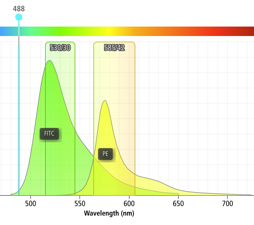
As you can see, something like 12% of the FITC fluorescence ends up in the PE channel!

Fortunately, a little linear algebra can fix this problem, and Cytoflow makes it easy. However, you’ll need to run a few controls:

• A blank control – one with your cells but without any fluorophores. This will let us measure the “background” fluorescence (or autofluorescence) of the samples.

• A set of single-color controls – for each fluorophore, one control that is stained with (or expresses) only that fluorophore and no others. These let us measure how much signal “bleeds through” into the non-target channels. These controls should be as bright as (but no brigher than) your brightest experimental sample.

Warning

These controls must be collected using the SAME instrument settings as your experimental samples. It’s really best if they’re collected at the SAME TIME as your experimental samples – even properly calibrated instruments are known to drift substantially between days, or even over the course of a single day. And yes, that means you really should run these controls for every experiment. If you’d like a way to correct for day-to-day variability, see HOWTO: Use beads to correct for day-to-day variation.

Procedure

1. Collect the controls listed above.

2. Import your data into Cytoflow. Do not import your control samples (unless they’re part of the experiment.) In the example below, we’ll have three fluorescence channels – Pacific Blue-A, FITC-A and PE-Tx-Red-YG-A – in addition to the forward and side-scatter channels.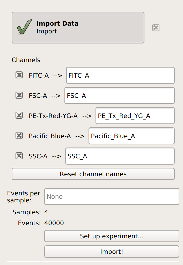

   

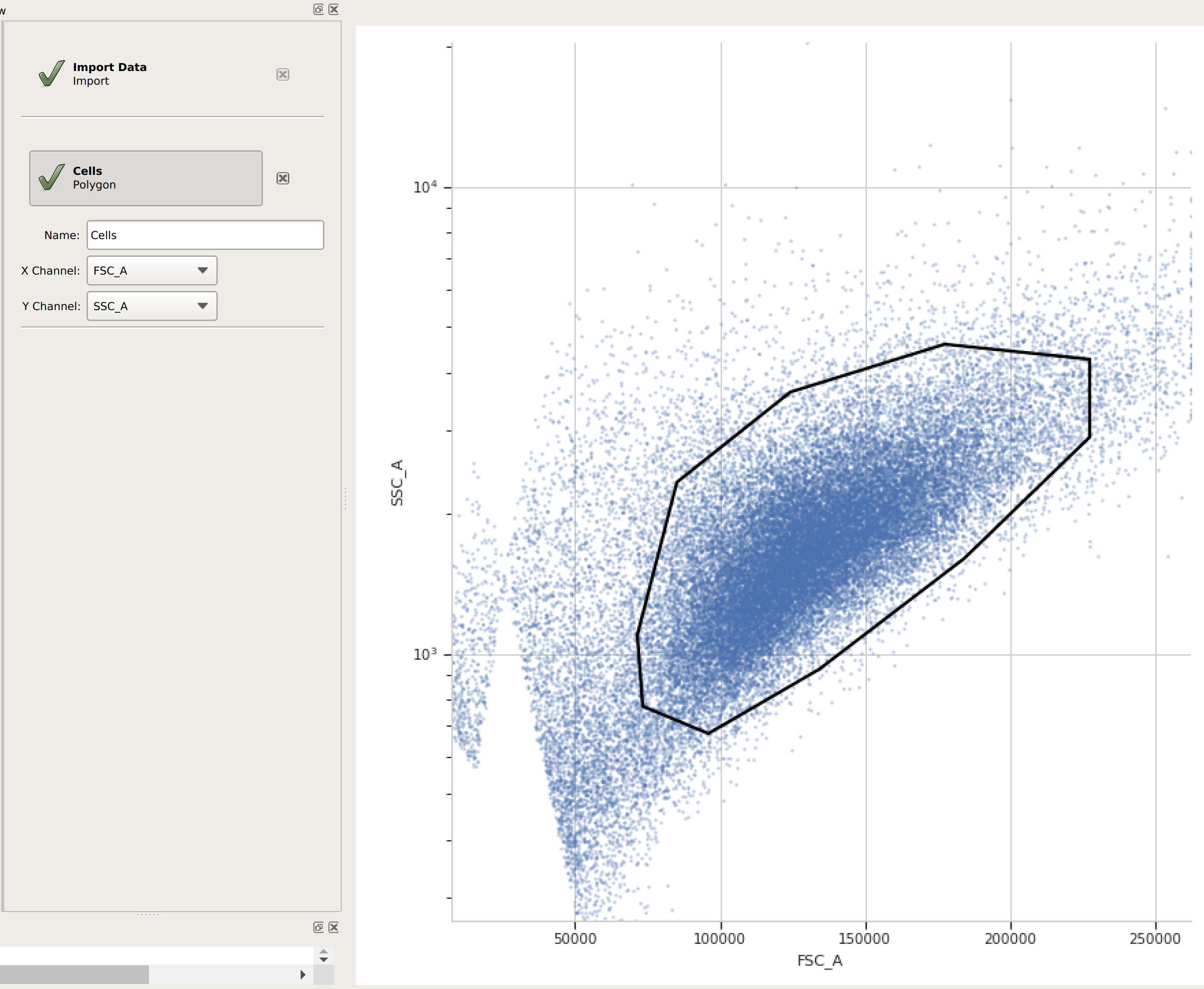
3. (Optional but recommended) - use a gate to filter out the “real” cells from debris and clumps. Here, I’m using a polygon gate on the foward-scatter and side-scatter channels to select the population of “real” cells. (I’ve named the population “Cells” – that’s how we’ll refer to it subsequently.

   

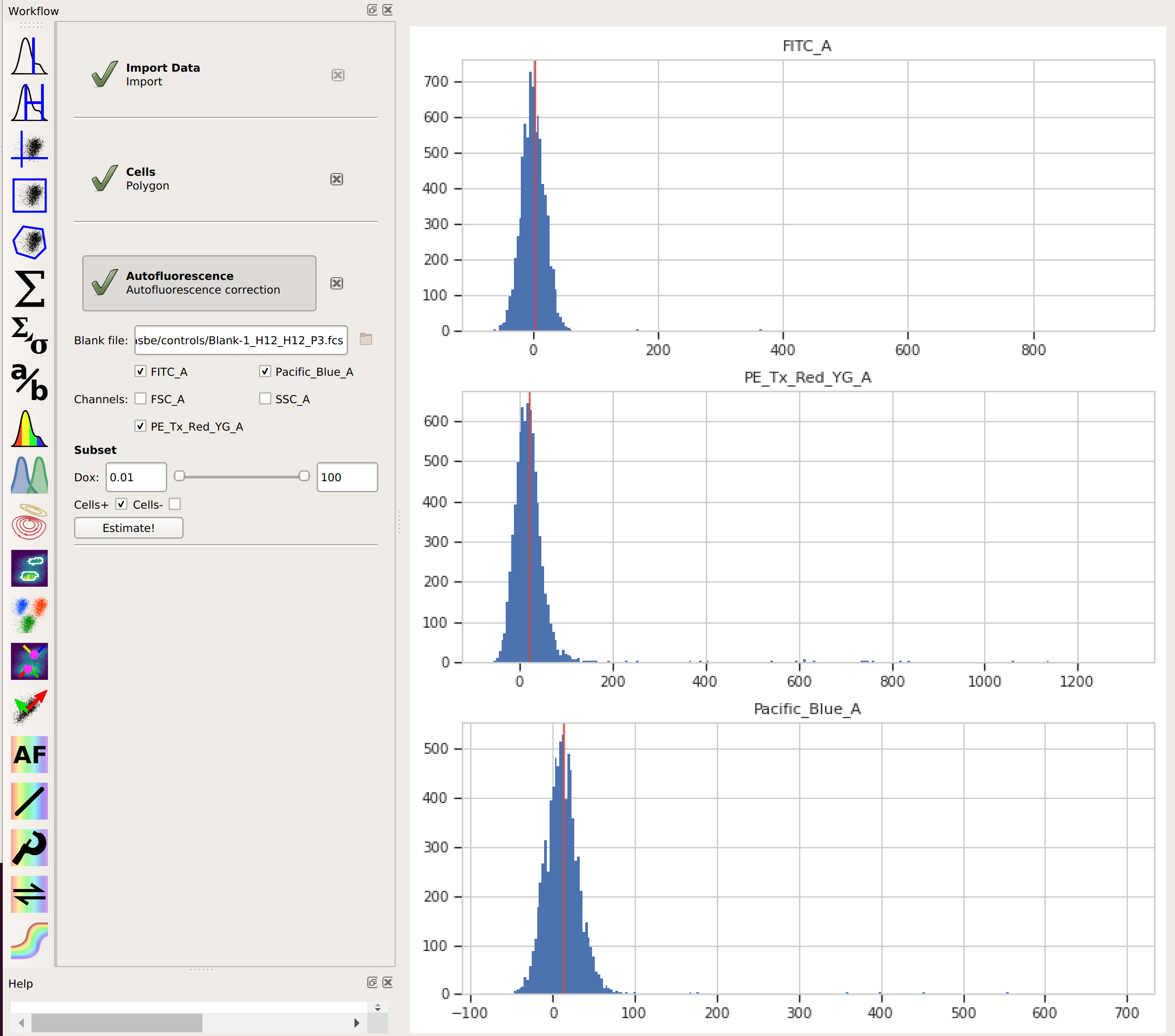
4. Add the Autofluorescence operation (it’s the button). Specify the file containing the data from the blank control, choose the channels you want to apply the correction to, and (if you followed the optional step above) choose the subset that you want to use to estimate the correction from. Once you’re done, click Estimate!

   The diagnostic plot shows a histogram of the fluorescence values from the blank file, and the red line indicates their median. This is the amount of “autofluorescence” that will be subtracted from your experimental data.

   

   Note

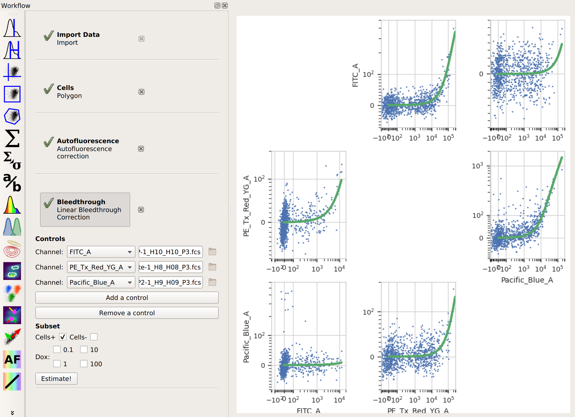
   By choosing the “Cells” subset, I told Cytoflow to apply the same gate from that operation to the blank data before estimating the autofluorescence correction. This way, the clumps and debris in the sample don’t influence that estimate. We’ll do the same thing in the next step, when we apply the bleedthrough compensation.

5. Add the Bleedthrough operation (it’s the button). For each control you have, click Add Control. In the Controls list, choose the channel you’re correcting and the file that contains the control data. Again, if you followed the optional step, also choose the subset you want to estimate the correction from. Then, click Estimate!.

   Here, the diagnostic plots show the data in the control files and the estimate that was fit to them. Because it’s a linear estimate, but the data is plotted on a logarithmic scale, the estimate lines are shown as curves.

   

And that’s it. Now you can continue on with your analysis, secure in the knowledge that you’ve successfully separated the adjacent fluorescence channels.

If you’d like to learn more, Abcam has a good page about compensation, and Mario Roederer has an even more detailed treatment.