cytoflow.operations.kmeans#
Use k-means clustering to cluster events in any number of dimensions.
kmeans has three classes:
KMeansOp – the IOperation to perform the clustering.
KMeans1DView – a diagnostic view of the clustering (1D, using a histogram)
KMeans2DView – a diagnostic view of the clustering (2D, using a scatterplot)
- class cytoflow.operations.kmeans.KMeansOp[source]#
Bases:
HasStrictTraitsUse a K-means clustering algorithm to cluster events.
Call
estimateto compute the cluster centroids.Calling
applycreates a new categorical metadata variable named{name}, with possible values0….n - 1wherenis the number of clusters, specified withnum_clusters.The same model may not be appropriate for different subsets of the data set. If this is the case, you can use the
byattribute to specify metadata by which to aggregate the data before estimating (and applying) a model. The number of clusters is the same across each subset, though.- name#
The operation name; determines the name of the new metadata column
- Type:
Str
- channels#
The channels to apply the clustering algorithm to.
- Type:
List(Str)
- scale#
Re-scale the data in the specified channels before fitting. If a channel is in
channelsbut not inscale, the current package-wide default (set withset_default_scale) is used.Note
Sometimes you may see events labeled
{name}_None– this results from events for which the selected scale is invalid. For example, if an event has a negative measurement in a channel and that channel’s scale is set to “log”, this event will be set to{name}_None.- Type:
Dict(Str : {“linear”, “logicle”, “log”})
- num_clusters#
How many components to fit to the data? Must be greater or equal to 2.
- Type:
Int
- by#
A list of metadata attributes to aggregate the data before estimating the model. For example, if the experiment has two pieces of metadata,
TimeandDox, settingbyto["Time", "Dox"]will fit the model separately to each subset of the data with a unique combination ofTimeandDox.- Type:
List(Str)
- Statistics#
- ----------
- Adds a statistic whose name is the name of the operation, whose columns are
- the channels used for clustering, and whose values are the centroids for
- each cluster in that channel. Useful for hierarchical clustering, minimum
- spanning tree visualizations, etc. The index has levels from `by`, plus a
- new level called ``Cluster``.
- The new statistic also has a feature named ``Proportion``, which has the
- proportion of events in each cluster.
Examples
Make a little data set.
>>> import cytoflow as flow
>>> import_op = flow.ImportOp()
>>> import_op.tubes = [flow.Tube(file = "Plate01/RFP_Well_A3.fcs",
...                              conditions = {'Dox' : 10.0}),
...                    flow.Tube(file = "Plate01/CFP_Well_A4.fcs",
...                              conditions = {'Dox' : 1.0})]
>>> import_op.conditions = {'Dox' : 'float'}
>>> ex = import_op.apply()
Create and parameterize the operation.
>>> km_op = flow.KMeansOp(name = 'KMeans',
...                       channels = ['V2-A', 'Y2-A'],
...                       scale = {'V2-A' : 'log',
...                                'Y2-A' : 'log'},
...                       num_clusters = 2)
Estimate the clusters
>>> km_op.estimate(ex)
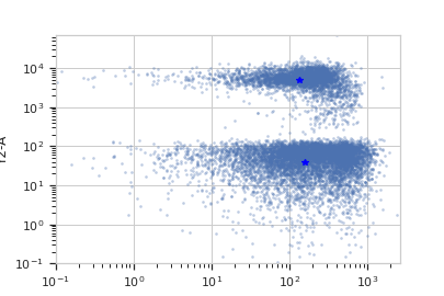
Plot a diagnostic view
>>> km_op.default_view().plot(ex)
Apply the gate
>>> ex2 = km_op.apply(ex)
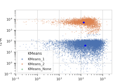
Plot a diagnostic view with the event assignments
>>> km_op.default_view().plot(ex2)
- estimate(experiment, subset=None)[source]#
Estimate the k-means clusters
- Parameters:
experiment (Experiment) – The
Experimentto use to estimate the k-means clusterssubset (str (default = None)) – A Python expression that specifies a subset of the data in
experimentto use to parameterize the operation.
- apply(experiment)[source]#
Apply the KMeans clustering to the data.
- Returns:
a new Experiment with one additional entry in
Experiment.conditionsnamedname, of typecategory. The new category has valuesname_1,name_2, etc to indicate which k-means cluster an event is a member of.The new
Experimentalso has one new statistic calledcenters, which is a list of tuples encoding the centroids of each k-means cluster.- Return type:
- default_view(**kwargs)[source]#
Returns a diagnostic plot of the k-means clustering.
- Returns:
IView
- Return type:
an IView, call
KMeans1DView.plotto see the diagnostic plot.
- class cytoflow.operations.kmeans.KMeans1DView[source]#
Bases:
By1DView,AnnotatingView,HistogramViewA diagnostic view for
KMeansOp(1D, using a histogram)- facets#
A read-only list of the conditions used to facet this view.
- Type:
List(Str)
- by#
A read-only list of the conditions used to group this view’s data before plotting.
- Type:
List(Str)
- channel#
The channel this view is viewing. If you created the view using
default_view, this is already set.- Type:
Str
- scale#
The way to scale the x axes. If you created the view using
default_view, this may be already set.- Type:
{‘linear’, ‘log’, ‘logicle’}
- subset#
An expression that specifies the subset of the statistic to plot. Passed unmodified to
pandas.DataFrame.query.- Type:
- xfacet#
Set to one of the
Experiment.conditionsin theExperiment, and a new column of subplots will be added for every unique value of that condition.- Type:
String
- yfacet#
Set to one of the
Experiment.conditionsin theExperiment, and a new row of subplots will be added for every unique value of that condition.- Type:
String
- huefacet#
Set to one of the
Experiment.conditionsin the in theExperiment, and a new color will be added to the plot for every unique value of that condition.- Type:
String
- plot(experiment, **kwargs)[source]#
Plot the plots.
- Parameters:
experiment (Experiment) – The
Experimentto plot using this view.title (str) – Set the plot title
xlabel (str) – Set the X axis label
ylabel (str) – Set the Y axis label
huelabel (str) – Set the label for the hue facet (in the legend)
legend (bool) – Plot a legend for the color or hue facet? Defaults to
True.legend_loc (str) – If we plot a legend, where should it go? This is a
matplotliblegend location string, like ‘lower right’ or ‘outside center right’. Default is ‘upper right’.sharex (bool) – If there are multiple subplots, should they share X axes? Defaults to
True.sharey (bool) – If there are multiple subplots, should they share Y axes? Defaults to
True.row_order (list) – Override the row facet value order with the given list. If a value is not given in the ordering, it is not plotted. Defaults to a “natural ordering” of all the values.
col_order (list) – Override the column facet value order with the given list. If a value is not given in the ordering, it is not plotted. Defaults to a “natural ordering” of all the values.
hue_order (list) – Override the hue facet value order with the given list. If a value is not given in the ordering, it is not plotted. Defaults to a “natural ordering” of all the values.
height (float) – The height of each row in inches. Default = 3.0
aspect (float) – The aspect ratio of each subplot. Default = 1.5
col_wrap (int) – If
xfacetis set andyfacetis not set, you can “wrap” the subplots around so that they form a multi-row grid by setting this to the number of columns you want.sns_style ({“darkgrid”, “whitegrid”, “dark”, “white”, “ticks”}) – Which
seabornstyle to apply to the plot? Default iswhitegrid.sns_context ({“notebook”, “paper”, “talk”, “poster”}) – Which
seaborncontext to use? Controls the scaling of plot elements such as tick labels and the legend. Default isnotebook.palette (palette name, list, or dict) – Colors to use for the different levels of the hue variable. Should be something that can be interpreted by
seaborn.color_palette, or a dictionary mapping hue levels to matplotlib colors. See https://seaborn.pydata.org/tutorial/color_palettes.html for a good overview.despine (Bool) – Remove the top and right axes from the plot? Default is
True.min_quantile (float (>0.0 and <1.0, default = 0.001)) – Clip data that is less than this quantile.
max_quantile (float (>0.0 and <1.0, default = 1.00)) – Clip data that is greater than this quantile.
lim ((float, float)) – Set the range of the plot’s data axis.
orientation ({‘vertical’, ‘horizontal’})
num_bins (int) – The number of bins to plot in the histogram. Clipped to [100, 1000]
histtype ({‘stepfilled’, ‘step’, ‘bar’}) – The type of histogram to draw.
stepfilledis the default, which is a line plot with a color filled under the curve.density (bool) – If
True, re-scale the histogram to form a probability density function, so the area under the histogram is 1.linewidth (float) – The width of the histogram line (in points)
linestyle ([‘-’ | ‘–’ | ‘-.’ | ‘:’ | “None”]) – The style of the line to plot
alpha (float (default = 0.5)) – The alpha blending value, between 0 (transparent) and 1 (opaque).
color (matplotlib color) – The color to plot the annotations. Overrides the default color cycle.
plot_name (Str) – If this
IViewcan make multiple plots,plot_nameis the name of the plot to make. Must be one of the values retrieved fromenum_plots.
- class cytoflow.operations.kmeans.KMeans2DView[source]#
Bases:
By2DView,AnnotatingView,ScatterplotViewA diagnostic view for
KMeansOp(2D, using a scatterplot).- facets#
A read-only list of the conditions used to facet this view.
- Type:
List(Str)
- by#
A read-only list of the conditions used to group this view’s data before plotting.
- Type:
List(Str)
- xchannel#
The channels to use for this view’s X axis. If you created the view using
default_view, this is already set.- Type:
Str
- ychannel#
The channels to use for this view’s Y axis. If you created the view using
default_view, this is already set.- Type:
Str
- xscale#
The way to scale the x axis. If you created the view using
default_view, this may be already set.- Type:
{‘linear’, ‘log’, ‘logicle’}
- yscale#
The way to scale the y axis. If you created the view using
default_view, this may be already set.- Type:
{‘linear’, ‘log’, ‘logicle’}
- huechannel#
If set, color the points using a normed color scale. The norm function is set by
huescale, and the color palette can be changed by passing thepaletteparameter toplot.- Type:
Str
- subset#
An expression that specifies the subset of the statistic to plot. Passed unmodified to
pandas.DataFrame.query.- Type:
- xfacet#
Set to one of the
Experiment.conditionsin theExperiment, and a new column of subplots will be added for every unique value of that condition.- Type:
String
- yfacet#
Set to one of the
Experiment.conditionsin theExperiment, and a new row of subplots will be added for every unique value of that condition.- Type:
String
- huefacet#
Set to one of the
Experiment.conditionsin the in theExperiment, and a new color will be added to the plot for every unique value of that condition.- Type:
String
- plot(experiment, **kwargs)[source]#
Plot the plots.
- Parameters:
experiment (Experiment) – The
Experimentto plot using this view.title (str) – Set the plot title
xlabel (str) – Set the X axis label
ylabel (str) – Set the Y axis label
huelabel (str) – Set the label for the hue facet (in the legend)
legend (bool) – Plot a legend for the color or hue facet? Defaults to
True.legend_loc (str) – If we plot a legend, where should it go? This is a
matplotliblegend location string, like ‘lower right’ or ‘outside center right’. Default is ‘upper right’.sharex (bool) – If there are multiple subplots, should they share X axes? Defaults to
True.sharey (bool) – If there are multiple subplots, should they share Y axes? Defaults to
True.row_order (list) – Override the row facet value order with the given list. If a value is not given in the ordering, it is not plotted. Defaults to a “natural ordering” of all the values.
col_order (list) – Override the column facet value order with the given list. If a value is not given in the ordering, it is not plotted. Defaults to a “natural ordering” of all the values.
hue_order (list) – Override the hue facet value order with the given list. If a value is not given in the ordering, it is not plotted. Defaults to a “natural ordering” of all the values.
height (float) – The height of each row in inches. Default = 3.0
aspect (float) – The aspect ratio of each subplot. Default = 1.5
col_wrap (int) – If
xfacetis set andyfacetis not set, you can “wrap” the subplots around so that they form a multi-row grid by setting this to the number of columns you want.sns_style ({“darkgrid”, “whitegrid”, “dark”, “white”, “ticks”}) – Which
seabornstyle to apply to the plot? Default iswhitegrid.sns_context ({“notebook”, “paper”, “talk”, “poster”}) – Which
seaborncontext to use? Controls the scaling of plot elements such as tick labels and the legend. Default isnotebook.palette (palette name, list, or dict) – Colors to use for the different levels of the hue variable. Should be something that can be interpreted by
seaborn.color_palette, or a dictionary mapping hue levels to matplotlib colors. See https://seaborn.pydata.org/tutorial/color_palettes.html for a good overview.despine (Bool) – Remove the top and right axes from the plot? Default is
True.min_quantile (float (>0.0 and <1.0, default = 0.001)) – Clip data that is less than this quantile.
max_quantile (float (>0.0 and <1.0, default = 1.00)) – Clip data that is greater than this quantile.
xlim ((float, float)) – Set the range of the plot’s X axis.
ylim ((float, float)) – Set the range of the plot’s Y axis.
alpha (float (default = 0.25)) – The alpha blending value, between 0 (transparent) and 1 (opaque).
s (int (default = 2)) – The size in points^2.
marker (a matplotlib marker style, usually a string) – Specfies the glyph to draw for each point on the scatterplot. See matplotlib.markers for examples. Default: ‘o’
color (matplotlib color) – The color to plot the annotations. Overrides the default color cycle.
plot_name (Str) – If this
IViewcan make multiple plots,plot_nameis the name of the plot to make. Must be one of the values retrieved fromenum_plots.