cytoflow.operations.gaussian_2d

class cytoflow.operations.gaussian_2d.GaussianMixture2DOp

Bases: traits.has_traits.HasStrictTraits

This module fits a 2D Gaussian mixture model with a specified number of components to a pair of channels.

Warning

GaussianMixture2DOp is DEPRECATED and will be removed in a future release. It doesn’t correctly handle the case where an event is present in more than one component. Please use GaussianMixtureOp instead!

Creates a new categorical metadata variable named name, with possible values name_1 …. name_n where n is the number of components. An event is assigned to name_i category if it falls within sigma standard deviations of the component’s mean. If that is true for multiple categories (or if sigma is 0.0), the event is assigned to the category with the highest posterior probability. If the event doesn’t fall into any category, it is assigned to name_None.

As a special case, if num_components is 1 and sigma > 0.0, then the new condition is boolean, True if the event fell in the gate and False otherwise.

Optionally, if posteriors is True, this module will also compute the posterior probability of each event in its assigned component, returning it in a new colunm named {Name}_Posterior.

Finally, the same mixture model (mean and standard deviation) may not be appropriate for every subset of the data. If this is the case, you can use the by attribute to specify metadata by which to aggregate the data before estimating (and applying) a mixture model. The number of components is the same across each subset, though.

name

The operation name; determines the name of the new metadata column

Type:Str

xchannel

The X channel to apply the mixture model to.

Type:Str

ychannel

The Y channel to apply the mixture model to.

Type:Str

xscale

Re-scale the data on the X acis before fitting the data?

Type:{“linear”, “logicle”, “log”} (default = “linear”)

yscale

Re-scale the data on the Y axis before fitting the data?

Type:{“linear”, “logicle”, “log”} (default = “linear”)

num_components

How many components to fit to the data? Must be positive.

Type:Int (default = 1)

sigma

How many standard deviations on either side of the mean to include in each category? If an event is in multiple components, assign it to the component with the highest posterior probability. If sigma is 0.0, categorize all the data by assigning each event to the component with the highest posterior probability. Must be >= 0.0.

Type:Float (default = 0.0)

by

A list of metadata attributes to aggregate the data before estimating the model. For example, if the experiment has two pieces of metadata, Time and Dox, setting by to ["Time", "Dox"] will fit the model separately to each subset of the data with a unique combination of Time and Dox.

Type:List(Str)

posteriors

If True, add a column named {Name}_Posterior giving the posterior probability that the event is in the component to which it was assigned. Useful for filtering out low-probability events.

Type:Bool (default = False)

Examples

Make a little data set.

>>> import cytoflow as flow
>>> import_op = flow.ImportOp()
>>> import_op.tubes = [flow.Tube(file = "Plate01/RFP_Well_A3.fcs",
...                              conditions = {'Dox' : 10.0}),
...                    flow.Tube(file = "Plate01/CFP_Well_A4.fcs",
...                              conditions = {'Dox' : 1.0})]
>>> import_op.conditions = {'Dox' : 'float'}
>>> ex = import_op.apply()

Create and parameterize the operation.

>>> gm_op = flow.GaussianMixture2DOp(name = 'Flow',
...                          xchannel = 'V2-A',
...                          xscale = 'log',
...                          ychannel = 'Y2-A',
...                          yscale = 'log',
...                          num_components = 2)

Estimate the clusters

>>> gm_op.estimate(ex)

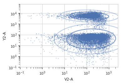
Plot a diagnostic view with the distributions

>>> gm_op.default_view().plot(ex)

Apply the gate

>>> ex2 = gm_op.apply(ex)

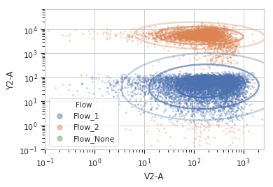
Plot a diagnostic view with the event assignments

>>> gm_op.default_view().plot(ex2)

estimate(experiment, subset=None)

Estimate the Gaussian mixture model parameters.

Parameters:

• experiment (Experiment) – The data to use to estimate the mixture parameters
• subset (str (default = None)) – If set, a Python expression to determine the subset of the data to use to in the estimation.

apply(experiment)

Assigns new metadata to events using the mixture model estimated in estimate().

Returns:A new Experiment with a column named name and optionally one named name _Posterior. Also includes the following new statistics:

• xmean : Float

  the mean of the fitted gaussian in the x dimension.

• ymean : Float

  the mean of the fitted gaussian in the y dimension.

• proportion : Float

  the proportion of events in each component of the mixture model. only set if num_components > 1.

PS – if someone has good ideas for summarizing spread in a 2D (non-isotropic) Gaussian, or other useful statistics, let me know!

Return type:Experiment

default_view(**kwargs)

Returns a diagnostic plot of the Gaussian mixture model.

Returns:

• IView (an IView, call plot() to see)
• the diagnostic plot.

class cytoflow.operations.gaussian_2d.GaussianMixture2DView

Bases: cytoflow.operations.base_op_views.By2DView, cytoflow.operations.base_op_views.AnnotatingView, cytoflow.views.scatterplot.ScatterplotView

A diagnostic plot for a GaussianMixture2DOp.

facets

A read-only list of the conditions used to facet this view.

Type:List(String)

by

A read-only list of the conditions used to group this view’s data before plotting.

Type:List(String)

xchannel, ychannel

The channels to use for this view’s X and Y axes. If you created the view using default_view(), this is already set.

Type:String

xscale, yscale

The way to scale the x axes. If you created the view using default_view(), this may be already set.

Type:{‘linear’, ‘log’, ‘logicle’}

op

The IOperation that this view is associated with. If you created the view using default_view(), this is already set.

Type:Instance(IOperation)

xlim, ylim

Set the min and max limits of the plots’ x and y axes.

Type:(float, float)

xfacet, yfacet

Set to one of the conditions in the Experiment, and a new row or column of subplots will be added for every unique value of that condition.

Type:String

huefacet

Set to one of the conditions in the in the Experiment, and a new color will be added to the plot for every unique value of that condition.

Type:String

huescale

How should the color scale for huefacet be scaled?

Type:{‘linear’, ‘log’, ‘logicle’}

plot(experiment, **kwargs)

Plot the plots.

Parameters:

• experiment (Experiment) – The Experiment to plot using this view.
• title (str) – Set the plot title
• xlabel, ylabel (str) – Set the X and Y axis labels
• huelabel (str) – Set the label for the hue facet (in the legend)
• legend (bool) – Plot a legend for the color or hue facet? Defaults to True.
• sharex, sharey (bool) – If there are multiple subplots, should they share axes? Defaults to True.
• height (float) – The height of each row in inches. Default = 3.0
• aspect (float) – The aspect ratio of each subplot. Default = 1.5
• col_wrap (int) – If xfacet is set and yfacet is not set, you can “wrap” the subplots around so that they form a multi-row grid by setting col_wrap to the number of columns you want.
• sns_style ({“darkgrid”, “whitegrid”, “dark”, “white”, “ticks”}) – Which seaborn style to apply to the plot? Default is whitegrid.
• sns_context ({“paper”, “notebook”, “talk”, “poster”}) – Which seaborn context to use? Controls the scaling of plot elements such as tick labels and the legend. Default is talk.
• despine (Bool) – Remove the top and right axes from the plot? Default is True.
• min_quantile (float (>0.0 and <1.0, default = 0.001)) – Clip data that is less than this quantile.
• max_quantile (float (>0.0 and <1.0, default = 1.00)) – Clip data that is greater than this quantile.
• xlim, ylim ((float, float)) – Set the range of the plot’s axis.
• alpha (float (default = 0.25)) – The alpha blending value, between 0 (transparent) and 1 (opaque).
• s (int (default = 2)) – The size in points^2.
• marker (a matplotlib marker style, usually a string) – Specfies the glyph to draw for each point on the scatterplot. See matplotlib.markers for examples. Default: ‘o’
• color (matplotlib color) – The color to plot the annotations. Overrides the default color cycle.
• plot_name (str) – If this IView can make multiple plots, plot_name is the name of the plot to make. Must be one of the values retrieved from enum_plots().