cytoflow.operations.gaussian#

gaussian contains three classes:

GaussianMixtureOp – an operation that fits a Gaussian mixture model to one or more channels.

GaussianMixture1DView – a diagnostic view that shows how the GaussianMixtureOp estimated its model (on a 1D data set, using a histogram).

GaussianMixture2DView – a diagnostic view that shows how the GaussianMixtureOp estimated its model (on a 2D data set, using a scatter plot).

class cytoflow.operations.gaussian.GaussianMixtureOp[source]#

Bases: HasStrictTraits

This module fits a Gaussian mixture model with a specified number of components to one or more channels.

If num_components > 1, apply creates a new categorical metadata variable named name, with possible values {name}_1 …. name_n where n is the number of components. An event is assigned to name_i category if it has the highest posterior probability of having been produced by component i. If an event has a value that is outside the range of one of the channels’ scales, then it is assigned to {name}_None.

Optionally, if sigma is greater than 0, apply creates new boolean metadata variables named {name}_1 … {name}_n where n is the number of components. The column {name}_i is True if the event is less than sigma standard deviations from the mean of component i. If num_components is 1, sigma must be greater than 0 and the new metadata name is the same as the operation name.

Note

The sigma attribute does NOT affect how events are assigned to components in the new name variable. That is to say, if an event is more than sigma standard deviations from ALL of the components, you might expect it would be labeled as {name}_None. It is not. An event is only labeled {name}_None if it has a value that is outside of the channels’ scales.

Optionally, if posteriors is True, apply creates a new double metadata variables named {name}_1_posterior … {name}_n_posterior where n is the number of components. The column {name}_i_posterior contains the posterior probability that this event is a member of component i.

Finally, the same mixture model (mean and standard deviation) may not be appropriate for every subset of the data. If this is the case, you can use the by attribute to specify metadata by which to aggregate the data before estimating (and applying) a mixture model. The number of components must be the same across each subset, though.

name#

The operation name; determines the name of the new metadata column

Type:: Str

channels#

The channels to apply the mixture model to.

Type:: List(Str)

scale#

Re-scale the data in the specified channels before fitting. If a channel is in channels but not in scale, the current package-wide default (set with set_default_scale) is used.

Type:: Dict(Str : {“linear”, “logicle”, “log”})

num_components#

How many components to fit to the data? Must be a positive integer.

Type:: Int (default = 1)

sigma#

If not None, use this operation as a “gate”: for each component, create a new boolean variable {name}_i and if the event is within sigma standard deviations, set that variable to True. If num_components is 1, must be > 0.

Type:: Float

by#

A list of metadata attributes to aggregate the data before estimating the model. For example, if the experiment has two pieces of metadata, Time and Dox, setting by to ["Time", "Dox"] will fit the model separately to each subset of the data with a unique combination of Time and Dox.

Type:: List(Str)

posteriors#

If True, add columns named {name}_{i}_posterior giving the posterior probability that the event is in component i. Useful for filtering out low-probability events.

Type:: Bool (default = False)

Statistics#

----------

Calling `apply` adds a statistic with the following columns to the returned `Experiment`.

.. important::: If num_components is greater than 1, Component is added as another level to the statistic index.

- **{{Channel}} Mean**

for each component.

Type:: The mean of the fitted gaussian in each channel

- **{{Channel}} SD**

rescaled with the channel scale

Type:: The standard deviation of the fitted gaussian,

- **{{Channel}} Interval Low**

rescaled for the channel scale

Type:: The mean minus the standard deviation,

- **{{Channel}} Interval High**

rescaled for the channel scale

Type:: The mean plus the standard deviation,

- **Proportion**

added if num_components is greater than 1.

Type:: The proportion of events in each component of the mixture model. Only

Notes

We use the Mahalnobis distance as a multivariate generalization of the number of standard deviations an event is from the mean of the multivariate gaussian. If \(\vec{x}\) is an observation from a distribution with mean \(\vec{\mu}\) and \(S\) is the covariance matrix, then the Mahalanobis distance is \(\sqrt{(x - \mu)^T \cdot S^{-1} \cdot (x - \mu)}\).

Examples

Make a little data set.

>>> import cytoflow as flow
>>> import_op = flow.ImportOp()
>>> import_op.tubes = [flow.Tube(file = "Plate01/RFP_Well_A3.fcs",
...                              conditions = {'Dox' : 10.0}),
...                    flow.Tube(file = "Plate01/CFP_Well_A4.fcs",
...                              conditions = {'Dox' : 1.0})]
>>> import_op.conditions = {'Dox' : 'float'}
>>> ex = import_op.apply()

Create and parameterize the operation.

>>> gm_op = flow.GaussianMixtureOp(name = 'Gauss',
...                                channels = ['Y2-A'],
...                                scale = {'Y2-A' : 'log'},
...                                num_components = 2)

Estimate the clusters

>>> gm_op.estimate(ex)

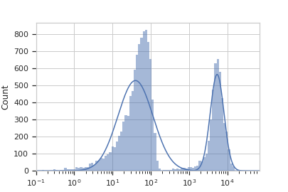
Plot a diagnostic view

>>> gm_op.default_view().plot(ex)

../../_images/cytoflow-operations-gaussian-4.png

Apply the gate

>>> ex2 = gm_op.apply(ex)

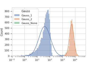
Plot a diagnostic view with the event assignments

>>> gm_op.default_view().plot(ex2)

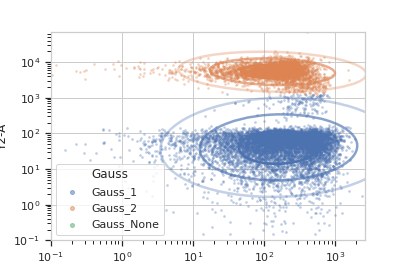
../../_images/cytoflow-operations-gaussian-6.png

And with two channels:

>>> gm_op = flow.GaussianMixtureOp(name = 'Gauss',
...                                channels = ['V2-A', 'Y2-A'],
...                                scale = {'V2-A' : 'log',
...                                         'Y2-A' : 'log'},
...                                num_components = 2)
>>> gm_op.estimate(ex)
>>> ex2 = gm_op.apply(ex)
>>> gm_op.default_view().plot(ex2)

../../_images/cytoflow-operations-gaussian-7.png

estimate(experiment, subset=None)[source]#

Estimate the Gaussian mixture model parameters

Parameters:

experiment (Experiment) – The data to use to estimate the mixture parameters
subset (str (default = None)) – If set, a Python expression to determine the subset of the data to use to in the estimation.

apply(experiment)[source]#

Assigns new metadata to events using the mixture model estimated in estimate.

Returns:

A new Experiment with the new condition variables as described in the class documentation. Also adds the following new statistics:

{{Channel}} Mean
the mean of the fitted gaussian in each channel for each component.
{{Channel}} SD
The standard deviation of each channel for each component.
{{Channel}} - {{Channel}} Correlation
The correlation coefficient between each pair of channels for each component.
{{Channel}} ProportionFloat
the proportion of events in each component of the mixture model. only added if num_components > 1.

Return type:

Experiment

default_view(**kwargs)[source]#

Returns a diagnostic plot of the Gaussian mixture model.

Returns:: An IView, call plot to see the diagnostic plot.
Return type:: IView

class cytoflow.operations.gaussian.GaussianMixture1DView[source]#

Bases: By1DView, AnnotatingView, HistogramView

A default view for GaussianMixtureOp that plots the histogram of a single channel, then the estimated Gaussian distributions on top of it.

facets#

A read-only list of the conditions used to facet this view.

Type:: List(Str)

by#

A read-only list of the conditions used to group this view’s data before plotting.

Type:: List(Str)

channel#

The channel this view is viewing. If you created the view using default_view, this is already set.

Type:: Str

scale#

The way to scale the x axes. If you created the view using default_view, this may be already set.

Type:: {‘linear’, ‘log’, ‘logicle’}

op#

The IOperation that this view is associated with. If you created the view using default_view, this is already set.

Type:: Instance(IOperation)

subset#

An expression that specifies the subset of the statistic to plot. Passed unmodified to pandas.DataFrame.query.

Type:: str

xfacet#

Set to one of the Experiment.conditions in the Experiment, and a new column of subplots will be added for every unique value of that condition.

Type:: String

yfacet#

Set to one of the Experiment.conditions in the Experiment, and a new row of subplots will be added for every unique value of that condition.

Type:: String

huefacet#

Set to one of the Experiment.conditions in the in the Experiment, and a new color will be added to the plot for every unique value of that condition.

Type:: String

huescale#

How should the color scale for huefacet be scaled?

Type:: {‘linear’, ‘log’, ‘logicle’}

plot(experiment, **kwargs)[source]#

Plot the plots.

Parameters:

experiment (Experiment) – The Experiment to plot using this view.
title (str) – Set the plot title
xlabel (str) – Set the X axis label
ylabel (str) – Set the Y axis label
huelabel (str) – Set the label for the hue facet (in the legend)
legend (bool) – Plot a legend for the color or hue facet? Defaults to True.
legend_out (bool) – Plot the legend outside of the plot or grid? Defaults to True.
sharex (bool) – If there are multiple subplots, should they share X axes? Defaults to True.
sharey (bool) – If there are multiple subplots, should they share Y axes? Defaults to True.
row_order (list) – Override the row facet value order with the given list. If a value is not given in the ordering, it is not plotted. Defaults to a “natural ordering” of all the values.
col_order (list) – Override the column facet value order with the given list. If a value is not given in the ordering, it is not plotted. Defaults to a “natural ordering” of all the values.
hue_order (list) – Override the hue facet value order with the given list. If a value is not given in the ordering, it is not plotted. Defaults to a “natural ordering” of all the values.
height (float) – The height of each row in inches. Default = 3.0
aspect (float) – The aspect ratio of each subplot. Default = 1.5
col_wrap (int) – If xfacet is set and yfacet is not set, you can “wrap” the subplots around so that they form a multi-row grid by setting this to the number of columns you want.
sns_style ({“darkgrid”, “whitegrid”, “dark”, “white”, “ticks”}) – Which seaborn style to apply to the plot? Default is whitegrid.
sns_context ({“notebook”, “paper”, “talk”, “poster”}) – Which seaborn context to use? Controls the scaling of plot elements such as tick labels and the legend. Default is notebook.
palette (palette name, list, or dict) – Colors to use for the different levels of the hue variable. Should be something that can be interpreted by seaborn.color_palette, or a dictionary mapping hue levels to matplotlib colors. See https://seaborn.pydata.org/tutorial/color_palettes.html for a good overview.
despine (Bool) – Remove the top and right axes from the plot? Default is True.
min_quantile (float (>0.0 and <1.0, default = 0.001)) – Clip data that is less than this quantile.
max_quantile (float (>0.0 and <1.0, default = 1.00)) – Clip data that is greater than this quantile.
lim ((float, float)) – Set the range of the plot’s data axis.
orientation ({‘vertical’, ‘horizontal’})
num_bins (int) – The number of bins to plot in the histogram. Clipped to [100, 1000]
histtype ({‘stepfilled’, ‘step’, ‘bar’}) – The type of histogram to draw. stepfilled is the default, which is a line plot with a color filled under the curve.
density (bool) – If True, re-scale the histogram to form a probability density function, so the area under the histogram is 1.
linewidth (float) – The width of the histogram line (in points)
linestyle ([‘-’ | ‘–’ | ‘-.’ | ‘:’ | “None”]) – The style of the line to plot
alpha (float (default = 0.5)) – The alpha blending value, between 0 (transparent) and 1 (opaque).
color (matplotlib color) – The color to plot the annotations. Overrides the default color cycle.
plot_name (Str) – If this IView can make multiple plots, plot_name is the name of the plot to make. Must be one of the values retrieved from enum_plots.

cytoflow.operations.gaussian.poly_area(x, y)[source]#

class cytoflow.operations.gaussian.GaussianMixture2DView[source]#

Bases: By2DView, AnnotatingView, ScatterplotView

A default view for GaussianMixtureOp that plots the scatter plot of a two channels, then the estimated 2D Gaussian distributions on top of it.

facets#

A read-only list of the conditions used to facet this view.

Type:: List(Str)

by#

A read-only list of the conditions used to group this view’s data before plotting.

Type:: List(Str)

xchannel#

The channels to use for this view’s X axis. If you created the view using default_view, this is already set.

Type:: Str

ychannel#

The channels to use for this view’s Y axis. If you created the view using default_view, this is already set.

Type:: Str

xscale#

The way to scale the x axis. If you created the view using default_view, this may be already set.

Type:: {‘linear’, ‘log’, ‘logicle’}

yscale#

The way to scale the y axis. If you created the view using default_view, this may be already set.

Type:: {‘linear’, ‘log’, ‘logicle’}

op#

The IOperation that this view is associated with. If you created the view using default_view, this is already set.

Type:: Instance(IOperation)

huechannel#

If set, color the points using a normed color scale. The norm function is set by huescale, and the color palette can be changed by passing the palette parameter to plot.

Type:: Str

subset#

An expression that specifies the subset of the statistic to plot. Passed unmodified to pandas.DataFrame.query.

Type:: str

xfacet#

Set to one of the Experiment.conditions in the Experiment, and a new column of subplots will be added for every unique value of that condition.

Type:: String

yfacet#

Set to one of the Experiment.conditions in the Experiment, and a new row of subplots will be added for every unique value of that condition.

Type:: String

huefacet#

Set to one of the Experiment.conditions in the in the Experiment, and a new color will be added to the plot for every unique value of that condition.

Type:: String

huescale#

How should the color scale for huefacet be scaled?

Type:: {‘linear’, ‘log’, ‘logicle’}

plot(experiment, **kwargs)[source]#

Plot the plots.

Parameters:

experiment (Experiment) – The Experiment to plot using this view.
title (str) – Set the plot title
xlabel (str) – Set the X axis label
ylabel (str) – Set the Y axis label
huelabel (str) – Set the label for the hue facet (in the legend)
legend (bool) – Plot a legend for the color or hue facet? Defaults to True.
legend_out (bool) – Plot the legend outside of the plot or grid? Defaults to True.
sharex (bool) – If there are multiple subplots, should they share X axes? Defaults to True.
sharey (bool) – If there are multiple subplots, should they share Y axes? Defaults to True.
row_order (list) – Override the row facet value order with the given list. If a value is not given in the ordering, it is not plotted. Defaults to a “natural ordering” of all the values.
col_order (list) – Override the column facet value order with the given list. If a value is not given in the ordering, it is not plotted. Defaults to a “natural ordering” of all the values.
hue_order (list) – Override the hue facet value order with the given list. If a value is not given in the ordering, it is not plotted. Defaults to a “natural ordering” of all the values.
height (float) – The height of each row in inches. Default = 3.0
aspect (float) – The aspect ratio of each subplot. Default = 1.5
col_wrap (int) – If xfacet is set and yfacet is not set, you can “wrap” the subplots around so that they form a multi-row grid by setting this to the number of columns you want.
sns_style ({“darkgrid”, “whitegrid”, “dark”, “white”, “ticks”}) – Which seaborn style to apply to the plot? Default is whitegrid.
sns_context ({“notebook”, “paper”, “talk”, “poster”}) – Which seaborn context to use? Controls the scaling of plot elements such as tick labels and the legend. Default is notebook.
palette (palette name, list, or dict) – Colors to use for the different levels of the hue variable. Should be something that can be interpreted by seaborn.color_palette, or a dictionary mapping hue levels to matplotlib colors. See https://seaborn.pydata.org/tutorial/color_palettes.html for a good overview.
despine (Bool) – Remove the top and right axes from the plot? Default is True.
min_quantile (float (>0.0 and <1.0, default = 0.001)) – Clip data that is less than this quantile.
max_quantile (float (>0.0 and <1.0, default = 1.00)) – Clip data that is greater than this quantile.
xlim ((float, float)) – Set the range of the plot’s X axis.
ylim ((float, float)) – Set the range of the plot’s Y axis.
alpha (float (default = 0.25)) – The alpha blending value, between 0 (transparent) and 1 (opaque).
s (int (default = 2)) – The size in points^2.
marker (a matplotlib marker style, usually a string) – Specfies the glyph to draw for each point on the scatterplot. See matplotlib.markers for examples. Default: ‘o’
color (matplotlib color) – The color to plot the annotations. Overrides the default color cycle.
plot_name (Str) – If this IView can make multiple plots, plot_name is the name of the plot to make. Must be one of the values retrieved from enum_plots.