Statistics in cytoflow
One of the most powerful concepts in cytoflow is that it makes it
easy to summarize your data, then track how those subsets change as your
experimental variables change. This notebook demonstrates several
different modules that create and plot statistics.
Set up the Jupyter matplotlib integration, and import the
cytoflow module.
# in some buggy versions of the Jupyter notebook, this needs to be in its OWN CELL.
%matplotlib inline
import cytoflow as flow

# if your figures are too big or too small, you can scale them by changing matplotlib's DPI
import matplotlib
matplotlib.rc('figure', dpi = 160)
We use the same data set as the Yeast Dose Response example notebook, with one variant: we load each tube three times, grabbing only 100 events from each.
inputs = {
    "Yeast_B1_B01.fcs" : 5.0,
    "Yeast_B2_B02.fcs" : 3.75,
    "Yeast_B3_B03.fcs" : 2.8125,
    "Yeast_B4_B04.fcs" : 2.109,
    "Yeast_B5_B05.fcs" : 1.5820,
    "Yeast_B6_B06.fcs" : 1.1865,
    "Yeast_B7_B07.fcs" : 0.8899,
    "Yeast_B8_B08.fcs" : 0.6674,
    "Yeast_B9_B09.fcs" : 0.5,
    "Yeast_B10_B10.fcs" : 0.3754,
    "Yeast_B11_B11.fcs" : 0.2816,
    "Yeast_B12_B12.fcs" : 0.2112,
    "Yeast_C1_C01.fcs" : 0.1584,
    "Yeast_C2_C02.fcs" : 0.1188,
    "Yeast_C3_C03.fcs" : 0.0892,
    "Yeast_C4_C04.fcs" : 0.0668,
    "Yeast_C5_C05.fcs" : 0.05,
    "Yeast_C6_C06.fcs" : 0.0376,
    "Yeast_C7_C07.fcs" : 0.0282,
    "Yeast_C8_C08.fcs" : 0.0211,
    "Yeast_C9_C09.fcs" : 0.0159
}

tubes = []
for filename, ip in inputs.items():
    tubes.append(flow.Tube(file = "data/" + filename, conditions = {'IP' : ip, 'Replicate' : 1}))
    tubes.append(flow.Tube(file = "data/" + filename, conditions = {'IP' : ip, 'Replicate' : 2}))
    tubes.append(flow.Tube(file = "data/" + filename, conditions = {'IP' : ip, 'Replicate' : 3}))


ex = flow.ImportOp(conditions = {'IP' : "float", "Replicate" : "int"},
                   tubes = tubes,
                   events = 100).apply()
In cytoflow, a statistic is a value that summarizes something
about some data. cytoflow makes it easy to compute statistics for
various subsets. For example, if we expect the geometric mean of
FITC-A channel to change as the IP variable changes, we can
compute the geometric mean of the FITC-A channel of each different
IP condition with the ChannelStatisticOp operation:
op = flow.ChannelStatisticOp(name = "ByIP",
                             by = ["IP"],
                             channel = "FITC-A",
                             function = flow.geom_mean)
ex2 = op.apply(ex)
This operation splits the data set by different values of IP, then
applies the function flow.geom_mean to the FITC-A channel in
each subset. The result is stored in the statistics attribute of an
Experiment. The statistics attribute is a dictionary. The keys
are tuples, where the first element in the tuple is the name of the
operation that created the statistic, and the second element is specific
to the operation:
ex2.statistics.keys()
dict_keys([('ByIP', 'geom_mean')])
The Statistics1DOp operation sets the second element of the tuple to
the function name. (You can override this by setting
Statistics1DOp.statistic_name; this is useful if function is a
lambda function.)
The value of each entry in Experiment.statistics is a
pandas.Series. The series index is all the subsets for which the
statistic was computed, and the contents are the values of the statstic
itself.
ex2.statistics[('ByIP', 'geom_mean')]
IP
0.0159     106.760464
0.0211     145.242912
0.0282     152.152489
0.0376     194.243504
0.0500     240.788179
0.0668     413.218589
0.0892     670.798705
0.1188     971.121453
0.1584    1345.581190
0.2112    1203.016726
0.2816    1463.993731
0.3754    1733.702533
0.5000    1871.968527
0.6674    2218.190937
0.8899    2324.630935
1.1865    2486.103908
1.5820    2456.024025
2.1090    2326.584475
2.8125    2350.038991
3.7500    2676.275419
5.0000    2269.741514
Name: ByIP : geom_mean, dtype: float64
We can also specify multiple variables to break data set into. In the
example above, Statistics1DOp lumps all events with the same value
of IP together, but each amount of IP actually has three values
of Replicate as well. Let’s apply geom_mean to each unique
combination of IP and Replicate:
op = flow.ChannelStatisticOp(name = "ByIP",
                             by = ["IP", "Replicate"],
                             channel = "FITC-A",
                             function = flow.geom_mean)
ex2 = op.apply(ex)
ex2.statistics[("ByIP", "geom_mean")][0:12]
IP      Replicate
0.0159  1            109.294581
        2            106.956580
        3            104.099598
0.0211  1            144.564288
        2            147.712897
        3            143.484638
0.0282  1            155.558697
        2            156.508248
        3            144.679053
0.0376  1            182.294878
        2            206.147145
        3            195.023849
Name: ByIP : geom_mean, dtype: float64
Note that the pandas.Series now has a MultiIndex: there are
values for each unique combination of IP and Replicate.
Now that we have computed a statistic, we can plot it with one of the statistics views. We can use a bar chart:
flow.BarChartView(statistic = ("ByIP", "geom_mean"),
                  variable = "IP").plot(ex2)
---------------------------------------------------------------------------

CytoflowViewError                         Traceback (most recent call last)

<ipython-input-8-4102c59fbf66> in <module>
      1 flow.BarChartView(statistic = ("ByIP", "geom_mean"),
----> 2                   variable = "IP").plot(ex2)


~/src/cytoflow/cytoflow/views/bar_chart.py in plot(self, experiment, plot_name, **kwargs)
    129         """
    130
--> 131         super().plot(experiment, plot_name, **kwargs)
    132
    133     def _grid_plot(self, experiment, grid, **kwargs):


~/src/cytoflow/cytoflow/views/base_views.py in plot(self, experiment, plot_name, **kwargs)
    859                      plot_name = plot_name,
    860                      scale = scale,
--> 861                      **kwargs)
    862
    863     def _make_data(self, experiment):


~/src/cytoflow/cytoflow/views/base_views.py in plot(self, experiment, data, plot_name, **kwargs)
    712                                              "plot variables or the plot name. "
    713                                              "Possible plot names: {}"
--> 714                                              .format(unused_names, list(groupby.groups.keys())))
    715
    716             if plot_name not in set(groupby.groups.keys()):


CytoflowViewError: ('plot_name', "You must use facets ['Replicate'] in either the plot variables or the plot name. Possible plot names: [1, 2, 3]")
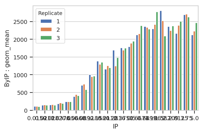
Oops! We forgot to specify how to plot the different Replicates.
Each index of a statistic must be specified as either a variable or a
facet of the plot, like so:
flow.BarChartView(statistic = ("ByIP", "geom_mean"),
                  variable = "IP",
                  huefacet = "Replicate").plot(ex2)
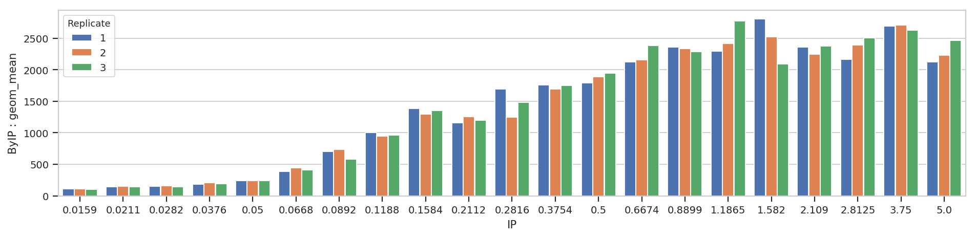
A quick aside - sometimes you get ugly axes because of overlapping
labels. In this case, we want a wider plot. While we can directly
specify the height of a plot, we can’t directly specify its width, only
its aspect ratio (the ratio of the width to the height.) cytoflow
defaults to 1.5; in this case, let’s widen it out to 4. If this results
in a plot that’s wider than your browser, the Jupyter notebook will
scale it down for you.
flow.BarChartView(statistic = ("ByIP", "geom_mean"),
                  variable = "IP",
                  huefacet = "Replicate").plot(ex2, aspect = 4)
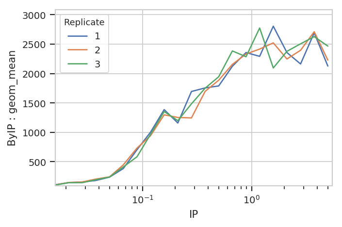
Bar charts are really best for categorical variables (with a modest number of categories.) Let’s do a line chart instead:
flow.Stats1DView(statistic = ("ByIP", "geom_mean"),
                 variable = "IP",
                 variable_scale = 'log',
                 huefacet = "Replicate").plot(ex2)
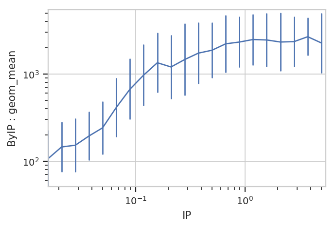
Statistics views can also plot error bars; the error bars must also be a statistic, and they must have the same indices as the “main” statistic. For example, let’s plot the geometric mean and geometric standard deviation of each IP subset:
ex2 = flow.ChannelStatisticOp(name = "ByIP",
                              by = ["IP"],
                              channel = "FITC-A",
                              function = flow.geom_mean).apply(ex)

# While an arithmetic SD is usually plotted plus-or-minus the arithmetic mean,
# a *geometric* SD is usually plotted (on a log scale!) multiplied-or-divided by the
# geometric mean.  the function geom_sd_range is a convenience function that does this.

ex3 = flow.ChannelStatisticOp(name = "ByIP",
                              by = ['IP'],
                              channel = "FITC-A",
                              function = flow.geom_sd_range).apply(ex2)

flow.Stats1DView(statistic = ("ByIP", "geom_mean"),
                 variable = "IP",
                 variable_scale = "log",
                 scale = "log",
                 error_statistic = ("ByIP", "geom_sd_range")).plot(ex3)
The plot above shows how one statistic varies (on the Y axis) as a variable changes on the X axis. We can also plot two statistics against eachother. For example, we can ask if the geometric standard deviation varies as the geometric mean changes:
ex2 = flow.ChannelStatisticOp(name = "ByIP",
                              by = ["IP"],
                              channel = "FITC-A",
                              function = flow.geom_mean).apply(ex)

ex3 = flow.ChannelStatisticOp(name = "ByIP",
                              by = ['IP'],
                              channel = "FITC-A",
                              function = flow.geom_sd).apply(ex2)

flow.Stats2DView(variable = "IP",
                 xstatistic = ("ByIP", "geom_mean"),
                 ystatistic = ("ByIP", "geom_sd"),
                 xscale = "log").plot(ex3)
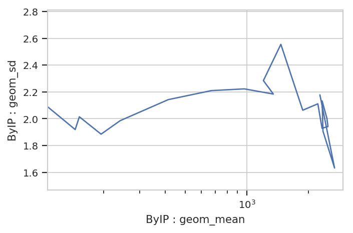
Nope, guess not. See the TASBE Calibrated Flow Cytometry notebook for more examples of 1D and 2D statistics views.
Transforming statistics
In addition to making statistics by applying summary functions to data,
you can also apply functions to other statistics. For example, a common
question is “What percentage of my events are in a particular gate?” We
could, for instance, ask what percentage of events are above 1000 in the
FITC-A channel, and how that varies by amount of IP. We start by
defining a threshold gate with ThresholdOp:
thresh = flow.ThresholdOp(name = "Above1000",
                          channel = "FITC-A",
                          threshold = 1000)
ex2 = thresh.apply(ex)
Now, the Experiment has a condition named Above1000 that is
True or False depending on whether that event’s FITC-A
channel is greater than 1000. Next, we compute the total number of
events in each subset with a unique combination of Above1000 and
IP:
ex3 = flow.ChannelStatisticOp(name = "Above1000",
                              by = ["Above1000", "IP"],
                              channel = "FITC-A",
                              function = len).apply(ex2)
ex3.statistics[("Above1000", "len")]
Above1000  IP
False      0.0159    299
           0.0211    299
           0.0282    299
           0.0376    296
           0.0500    299
           0.0668    262
           0.0892    200
           0.1188    143
           0.1584     76
           0.2112    101
           0.2816     76
           0.3754     57
           0.5000     53
           0.6674     32
           0.8899     19
           1.1865     23
           1.5820     21
           2.1090     34
           2.8125     25
           3.7500     10
           5.0000     29
True       0.0159      1
           0.0211      1
           0.0282      1
           0.0376      4
           0.0500      1
           0.0668     38
           0.0892    100
           0.1188    157
           0.1584    224
           0.2112    199
           0.2816    224
           0.3754    243
           0.5000    247
           0.6674    268
           0.8899    281
           1.1865    277
           1.5820    279
           2.1090    266
           2.8125    275
           3.7500    290
           5.0000    271
Name: Above1000 : len, dtype: int64
And now we compute the proportion of Above1000 == True for each
value of IP. TransformStatisticOp applies a function to subsets
of a statistic; in this case, we’re applying a lambda function to
convert each IP subset from length into proportion.
import pandas as pd

ex4 = flow.TransformStatisticOp(name = "Above1000",
                                statistic = ("Above1000", "len"),
                                by = ["IP"],
                                function = lambda a: pd.Series(a / a.sum()),
                                statistic_name = "proportion").apply(ex3)

ex4.statistics[("Above1000", "proportion")][0:8]
Above1000  IP
False      0.0159    0.996667
           0.0211    0.996667
           0.0282    0.996667
           0.0376    0.986667
           0.0500    0.996667
           0.0668    0.873333
           0.0892    0.666667
           0.1188    0.476667
Name: Above1000 : len, dtype: float64
Now we can plot the new statistic.
flow.Stats1DView(statistic = ("Above1000", "proportion"),
                 variable = "IP",
                 variable_scale = "log",
                 huefacet = "Above1000").plot(ex4)
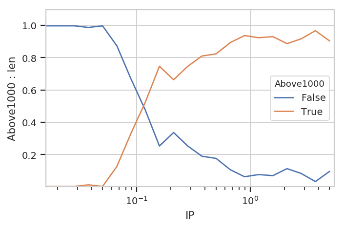
Note that be default we get all the values in the statistic; in this
case, it’s both the proportion that’s above 1000 (True) and the
proportion that is below it (False). We can pass a subset
attribute to the Stats1DView to look at just one or the other.
flow.Stats1DView(statistic = ("Above1000", "proportion"),
                 variable = "IP",
                 variable_scale = "log",
                 subset = "Above1000 == True").plot(ex4)
/home/brian/src/cytoflow/cytoflow/views/base_views.py:751: CytoflowViewWarning: Only one value for level Above1000; dropping it.
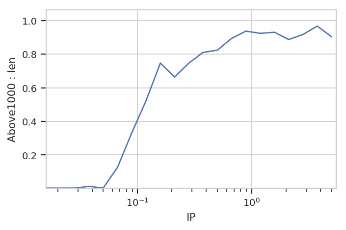
Note the warning. Because the index level Above1000 is always
True in this subset, it gets dropped from the index. Note also that
we don’t have to specify it as a variable or facet anywhere.
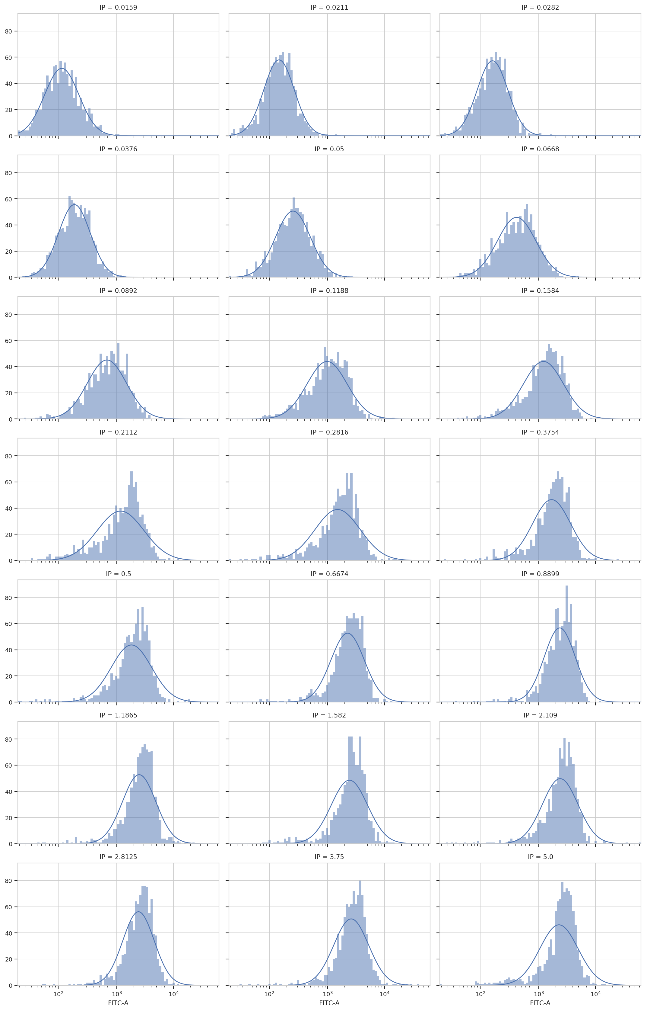
Statistics from data-driven modules
One of the most exciting aspects of statistics in cytoflow is that
other data-driven modules can add them to an Experiment, too. For
example, the GaussianMixtureOp adds several statistics for each
component of the mixture model it fits, containing the mean, standard
deviation and proportion of observations in each component:
inputs = {
    "Yeast_B1_B01.fcs" : 5.0,
    "Yeast_B2_B02.fcs" : 3.75,
    "Yeast_B3_B03.fcs" : 2.8125,
    "Yeast_B4_B04.fcs" : 2.109,
    "Yeast_B5_B05.fcs" : 1.5820,
    "Yeast_B6_B06.fcs" : 1.1865,
    "Yeast_B7_B07.fcs" : 0.8899,
    "Yeast_B8_B08.fcs" : 0.6674,
    "Yeast_B9_B09.fcs" : 0.5,
    "Yeast_B10_B10.fcs" : 0.3754,
    "Yeast_B11_B11.fcs" : 0.2816,
    "Yeast_B12_B12.fcs" : 0.2112,
    "Yeast_C1_C01.fcs" : 0.1584,
    "Yeast_C2_C02.fcs" : 0.1188,
    "Yeast_C3_C03.fcs" : 0.0892,
    "Yeast_C4_C04.fcs" : 0.0668,
    "Yeast_C5_C05.fcs" : 0.05,
    "Yeast_C6_C06.fcs" : 0.0376,
    "Yeast_C7_C07.fcs" : 0.0282,
    "Yeast_C8_C08.fcs" : 0.0211,
    "Yeast_C9_C09.fcs" : 0.0159
}

tubes = []
for filename, ip in inputs.items():
    tubes.append(flow.Tube(file = "data/" + filename, conditions = {'IP' : ip}))


ex = flow.ImportOp(conditions = {'IP' : "float"},
                   tubes = tubes).apply()
op = flow.GaussianMixtureOp(name = "Gauss",
                            channels = ["FITC-A"],
                            scale = {"FITC-A" : 'logicle'},
                            by = ["IP"],
                            num_components = 1)
op.estimate(ex)
ex2 = op.apply(ex)
op.default_view(xfacet = "IP").plot(ex2, col_wrap = 3)
ex2.statistics.keys()
dict_keys([('Gauss', 'mean'), ('Gauss', 'sigma'), ('Gauss', 'interval')])
ex2.statistics[("Gauss", 'mean')]
IP      Component  Channel
0.0159  1          FITC-A      114.867593
0.0211  1          FITC-A      146.760865
0.0282  1          FITC-A      161.831942
0.0376  1          FITC-A      188.241811
0.0500  1          FITC-A      252.533895
0.0668  1          FITC-A      415.359435
0.0892  1          FITC-A      675.335896
0.1188  1          FITC-A      976.574632
0.1584  1          FITC-A     1212.127491
0.2112  1          FITC-A     1169.357113
0.2816  1          FITC-A     1491.938821
0.3754  1          FITC-A     1683.611714
0.5000  1          FITC-A     1812.128528
0.6674  1          FITC-A     2233.860489
0.8899  1          FITC-A     2341.076532
1.1865  1          FITC-A     2474.300525
1.5820  1          FITC-A     2401.710245
2.1090  1          FITC-A     2383.285932
2.8125  1          FITC-A     2411.122019
3.7500  1          FITC-A     2584.007182
5.0000  1          FITC-A     2265.732416
Name: Gauss : mean, dtype: float64
ex2.statistics[("Gauss", 'interval')]
IP      Component  Channel
0.0159  1          FITC-A       (56.94459866110697, 224.1783518669721)
0.0211  1          FITC-A       (80.36534657785384, 265.7842407147643)
0.0282  1          FITC-A       (88.27508462690886, 295.4218184072569)
0.0376  1          FITC-A      (101.18497543667104, 350.4182139054138)
0.0500  1          FITC-A     (127.95204222704295, 502.06564927968213)
0.0668  1          FITC-A       (195.2351392293184, 894.5712089072493)
0.0892  1          FITC-A     (310.61832832262314, 1484.6617729462246)
0.1188  1          FITC-A       (437.6150673574889, 2200.017570462604)
0.1584  1          FITC-A      (542.1024597233911, 2732.4410991530126)
0.2112  1          FITC-A      (459.2685949581729, 3011.3302773605374)
0.2816  1          FITC-A      (601.1140138003304, 3736.1069195737864)
0.3754  1          FITC-A      (784.0312198090705, 3635.8937650247603)
0.5000  1          FITC-A       (802.3248292365361, 4117.843046843494)
0.6674  1          FITC-A      (1134.2954460750368, 4414.715040960627)
0.8899  1          FITC-A      (1246.7333023687233, 4408.716470275269)
1.1865  1          FITC-A        (1256.858649306397, 4886.57964348989)
1.5820  1          FITC-A      (1151.7297619649949, 5027.751372108821)
2.1090  1          FITC-A       (1161.983752683322, 4906.469724482335)
2.8125  1          FITC-A     (1276.8361886540924, 4566.1348774856815)
3.7500  1          FITC-A      (1277.3600413588333, 5244.721547284582)
5.0000  1          FITC-A      (1046.8993940886585, 4925.741101423763)
Name: Gauss : interval, dtype: object
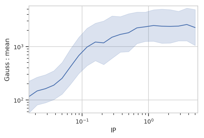
flow.Stats1DView(statistic = ("Gauss", "mean"),
                 variable = "IP",
                 variable_scale = "log",
                 scale = "log",
                 error_statistic = ("Gauss", "interval")).plot(ex2, shade_error = True)
/home/brian/src/cytoflow/cytoflow/views/base_views.py:751: CytoflowViewWarning: Only one value for level Component; dropping it.
/home/brian/src/cytoflow/cytoflow/views/base_views.py:751: CytoflowViewWarning: Only one value for level Channel; dropping it.