cytoflow.operations.kmeans
-
class
cytoflow.operations.kmeans.KMeansOp[source]¶ Bases:
traits.has_traits.HasStrictTraitsUse a K-means clustering algorithm to cluster events.
Call
estimate()to compute the cluster centroids.Calling
apply()creates a new categorical metadata variable namedname, with possible values{name}_1….name_nwherenis the number of clusters, specified withnum_clusters.The same model may not be appropriate for different subsets of the data set. If this is the case, you can use the
byattribute to specify metadata by which to aggregate the data before estimating (and applying) a model. The number of clusters is the same across each subset, though.-
name¶ The operation name; determines the name of the new metadata column
Type: Str
-
channels¶ The channels to apply the clustering algorithm to.
Type: List(Str)
-
scale¶ Re-scale the data in the specified channels before fitting. If a channel is in
channelsbut not inscale, the current package-wide default (set withset_default_scale()) is used.Type: Dict(Str : {“linear”, “logicle”, “log”})
-
num_clusters¶ How many components to fit to the data? Must be a positive integer.
Type: Int (default = 2)
-
by¶ A list of metadata attributes to aggregate the data before estimating the model. For example, if the experiment has two pieces of metadata,
TimeandDox, settingbyto["Time", "Dox"]will fit the model separately to each subset of the data with a unique combination ofTimeandDox.Type: List(Str)
Examples
Make a little data set.
>>> import cytoflow as flow
>>> import_op = flow.ImportOp()
>>> import_op.tubes = [flow.Tube(file = "Plate01/RFP_Well_A3.fcs",
...                              conditions = {'Dox' : 10.0}),
...                    flow.Tube(file = "Plate01/CFP_Well_A4.fcs",
...                              conditions = {'Dox' : 1.0})]
>>> import_op.conditions = {'Dox' : 'float'}
>>> ex = import_op.apply()
Create and parameterize the operation.
>>> km_op = flow.KMeansOp(name = 'KMeans',
...                       channels = ['V2-A', 'Y2-A'],
...                       scale = {'V2-A' : 'log',
...                                'Y2-A' : 'log'},
...                       num_clusters = 2)
Estimate the clusters
>>> km_op.estimate(ex)
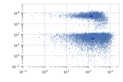
Plot a diagnostic view
>>> km_op.default_view().plot(ex)
Apply the gate
>>> ex2 = km_op.apply(ex)
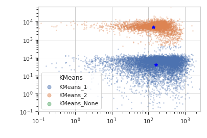
Plot a diagnostic view with the event assignments
>>> km_op.default_view().plot(ex2)
-
estimate(experiment, subset=None)[source]¶ Estimate the k-means clusters
Parameters: - experiment (Experiment) – The
Experimentto use to estimate the k-means clusters - subset (str (default = None)) – A Python expression that specifies a subset of the data in
experimentto use to parameterize the operation.
- experiment (Experiment) – The
-
apply(experiment)[source]¶ Apply the KMeans clustering to the data.
Returns: a new Experiment with one additional conditionnamedname, of typecategory. The new category has valuesname_1, name_2, etcto indicate which k-means cluster an event is a member of.The new
Experimentalso has one new statistic calledcenters, which is a list of tuples encoding the centroids of each k-means cluster.Return type: Experiment
-
default_view(**kwargs)[source]¶ Returns a diagnostic plot of the k-means clustering.
Returns: IView Return type: an IView, call KMeans1DView.plot()to see the diagnostic plot.
-
-
class
cytoflow.operations.kmeans.KMeans1DView[source]¶ Bases:
cytoflow.operations.base_op_views.By1DView,cytoflow.operations.base_op_views.AnnotatingView,cytoflow.views.histogram.HistogramView-
facets¶ A read-only list of the conditions used to facet this view.
Type: List(String)
-
by¶ A read-only list of the conditions used to group this view’s data before plotting.
Type: List(String)
-
channel¶ The channel this view is viewing. If you created the view using
default_view(), this is already set.Type: String
-
scale¶ The way to scale the x axes. If you created the view using
default_view(), this may be already set.Type: {‘linear’, ‘log’, ‘logicle’}
-
xfacet, yfacet Set to one of the
conditionsin theExperiment, and a new row or column of subplots will be added for every unique value of that condition.Type: String
-
huefacet¶ Set to one of the
conditionsin the in theExperiment, and a new color will be added to the plot for every unique value of that condition.Type: String
-
plot(experiment, **kwargs)[source]¶ Plot the plots.
Parameters: - experiment (Experiment) – The
Experimentto plot using this view. - title (str) – Set the plot title
- xlabel, ylabel (str) – Set the X and Y axis labels
- huelabel (str) – Set the label for the hue facet (in the legend)
- legend (bool) – Plot a legend for the color or hue facet? Defaults to True.
- sharex, sharey (bool) – If there are multiple subplots, should they share axes? Defaults to True.
- row_order, col_order, hue_order (list) – Override the row/column/hue facet value order with the given list. If a value is not given in the ordering, it is not plotted. Defaults to a “natural ordering” of all the values.
- height (float) – The height of each row in inches. Default = 3.0
- aspect (float) – The aspect ratio of each subplot. Default = 1.5
- col_wrap (int) – If xfacet is set and yfacet is not set, you can “wrap” the subplots around so that they form a multi-row grid by setting col_wrap to the number of columns you want.
- sns_style ({“darkgrid”, “whitegrid”, “dark”, “white”, “ticks”}) – Which seaborn style to apply to the plot? Default is whitegrid.
- sns_context ({“paper”, “notebook”, “talk”, “poster”}) – Which seaborn context to use? Controls the scaling of plot elements such as tick labels and the legend. Default is talk.
- despine (Bool) – Remove the top and right axes from the plot? Default is True.
- min_quantile (float (>0.0 and <1.0, default = 0.001)) – Clip data that is less than this quantile.
- max_quantile (float (>0.0 and <1.0, default = 1.00)) – Clip data that is greater than this quantile.
- lim ((float, float)) – Set the range of the plot’s data axis.
- orientation ({‘vertical’, ‘horizontal’})
- num_bins (int) – The number of bins to plot in the histogram. Clipped to [100, 1000]
- histtype ({‘stepfilled’, ‘step’, ‘bar’}) – The type of histogram to draw. stepfilled is the default, which is a line plot with a color filled under the curve.
- density (bool) – If True, re-scale the histogram to form a probability density function, so the area under the histogram is 1.
- linewidth (float) – The width of the histogram line (in points)
- linestyle ([‘-’ | ‘–’ | ‘-.’ | ‘:’ | “None”]) – The style of the line to plot
- alpha (float (default = 0.5)) – The alpha blending value, between 0 (transparent) and 1 (opaque).
- color (matplotlib color) – The color to plot the annotations. Overrides the default color cycle.
- plot_name (str) – If this
IViewcan make multiple plots,plot_nameis the name of the plot to make. Must be one of the values retrieved fromenum_plots().
- experiment (Experiment) – The
-
-
class
cytoflow.operations.kmeans.KMeans2DView[source]¶ Bases:
cytoflow.operations.base_op_views.By2DView,cytoflow.operations.base_op_views.AnnotatingView,cytoflow.views.scatterplot.ScatterplotView-
facets¶ A read-only list of the conditions used to facet this view.
Type: List(String)
-
by¶ A read-only list of the conditions used to group this view’s data before plotting.
Type: List(String)
-
xchannel, ychannel The channels to use for this view’s X and Y axes. If you created the view using
default_view(), this is already set.Type: String
-
xscale, yscale The way to scale the x axes. If you created the view using
default_view(), this may be already set.Type: {‘linear’, ‘log’, ‘logicle’}
-
xlim, ylim Set the min and max limits of the plots’ x and y axes.
Type: (float, float)
-
xfacet, yfacet Set to one of the
conditionsin theExperiment, and a new row or column of subplots will be added for every unique value of that condition.Type: String
-
huefacet¶ Set to one of the
conditionsin the in theExperiment, and a new color will be added to the plot for every unique value of that condition.Type: String
-
plot(experiment, **kwargs)[source]¶ Plot the plots.
Parameters: - experiment (Experiment) – The
Experimentto plot using this view. - title (str) – Set the plot title
- xlabel, ylabel (str) – Set the X and Y axis labels
- huelabel (str) – Set the label for the hue facet (in the legend)
- legend (bool) – Plot a legend for the color or hue facet? Defaults to True.
- sharex, sharey (bool) – If there are multiple subplots, should they share axes? Defaults to True.
- row_order, col_order, hue_order (list) – Override the row/column/hue facet value order with the given list. If a value is not given in the ordering, it is not plotted. Defaults to a “natural ordering” of all the values.
- height (float) – The height of each row in inches. Default = 3.0
- aspect (float) – The aspect ratio of each subplot. Default = 1.5
- col_wrap (int) – If xfacet is set and yfacet is not set, you can “wrap” the subplots around so that they form a multi-row grid by setting col_wrap to the number of columns you want.
- sns_style ({“darkgrid”, “whitegrid”, “dark”, “white”, “ticks”}) – Which seaborn style to apply to the plot? Default is whitegrid.
- sns_context ({“paper”, “notebook”, “talk”, “poster”}) – Which seaborn context to use? Controls the scaling of plot elements such as tick labels and the legend. Default is talk.
- despine (Bool) – Remove the top and right axes from the plot? Default is True.
- min_quantile (float (>0.0 and <1.0, default = 0.001)) – Clip data that is less than this quantile.
- max_quantile (float (>0.0 and <1.0, default = 1.00)) – Clip data that is greater than this quantile.
- xlim, ylim ((float, float)) – Set the range of the plot’s axis.
- alpha (float (default = 0.25)) – The alpha blending value, between 0 (transparent) and 1 (opaque).
- s (int (default = 2)) – The size in points^2.
- marker (a matplotlib marker style, usually a string) – Specfies the glyph to draw for each point on the scatterplot. See matplotlib.markers for examples. Default: ‘o’
- color (matplotlib color) – The color to plot the annotations. Overrides the default color cycle.
- plot_name (str) – If this
IViewcan make multiple plots,plot_nameis the name of the plot to make. Must be one of the values retrieved fromenum_plots().
- experiment (Experiment) – The
-