cytoflow.operations.binning

class cytoflow.operations.binning.BinningOp

Bases: traits.has_traits.HasStrictTraits

Bin data along an axis.

This operation creates equally spaced bins (in linear or log space) along an axis and adds a condition assigning each event to a bin. The value of the event’s condition is the left end of the bin’s interval in which the event is located.

name

The operation name. Used to name the new metadata field in the experiment that’s created by apply()

Type:Str

channel

The name of the channel along which to bin.

Type:Str

scale

Make the bins equidistant along what scale?

Type:{“linear”, “log”, “logicle”}

bin_width

The width of the bins. If scale is log, bin_width is in log-10 units; if scale is logicle, and error is thrown because the units are ill-defined.

Type:Float

Examples

Create a small experiment:

>>> import cytoflow as flow
>>> import_op = flow.ImportOp()
>>> import_op.tubes = [flow.Tube(file = "tasbe/rby.fcs")]
>>> ex = import_op.apply()

Create and parameterize the operation

>>> bin_op = flow.BinningOp()
>>> bin_op.name = "Bin"
>>> bin_op.channel = "FITC-A"
>>> bin_op.scale = "log"
>>> bin_op.bin_width = 0.2

Apply the operation to the experiment

>>> ex2 = bin_op.apply(ex)

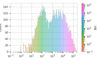
Plot the result

>>> bin_op.default_view().plot(ex2)

apply(experiment)

Applies the binning to an experiment.

Parameters:experiment (Experiment) – the old_experiment to which this op is applied Returns:A new experiment with a condition column named name, which contains the location of the left-most edge of the bin that the event is in. If bin_count_name is set, another column is added with that name as well, containing the number of events in the same bin as the event. Return type:Experiment

default_view(**kwargs)

Returns a diagnostic plot to check the binning.

Returns:An view instance, call plot() to plot the bins. Return type:IView

class cytoflow.operations.binning.BinningView

Bases: cytoflow.operations.base_op_views.Op1DView, cytoflow.operations.base_op_views.AnnotatingView, cytoflow.views.histogram.HistogramView

Plots a histogram of the current binning op. By default, the different bins are shown in different colors.

channel

The channel this view is viewing. If you created the view using default_view(), this is already set.

Type:String

scale

The way to scale the x axes. If you created the view using default_view(), this may be already set.

Type:{‘linear’, ‘log’, ‘logicle’}

op

The IOperation that this view is associated with. If you created the view using default_view(), this is already set.

Type:Instance(IOperation)

xfacet, yfacet

Set to one of the conditions in the Experiment, and a new row or column of subplots will be added for every unique value of that condition.

Type:String

huefacet

Set to one of the conditions in the in the Experiment, and a new color will be added to the plot for every unique value of that condition.

Type:String

huescale

How should the color scale for huefacet be scaled?

Type:{‘linear’, ‘log’, ‘logicle’}

plot(experiment, **kwargs)

Plot the histogram.

Parameters:

• experiment (Experiment) – The Experiment to plot using this view.
• title (str) – Set the plot title
• xlabel, ylabel (str) – Set the X and Y axis labels
• huelabel (str) – Set the label for the hue facet (in the legend)
• legend (bool) – Plot a legend for the color or hue facet? Defaults to True.
• sharex, sharey (bool) – If there are multiple subplots, should they share axes? Defaults to True.
• row_order, col_order, hue_order (list) – Override the row/column/hue facet value order with the given list. If a value is not given in the ordering, it is not plotted. Defaults to a “natural ordering” of all the values.
• height (float) – The height of each row in inches. Default = 3.0
• aspect (float) – The aspect ratio of each subplot. Default = 1.5
• col_wrap (int) – If xfacet is set and yfacet is not set, you can “wrap” the subplots around so that they form a multi-row grid by setting col_wrap to the number of columns you want.
• sns_style ({“darkgrid”, “whitegrid”, “dark”, “white”, “ticks”}) – Which seaborn style to apply to the plot? Default is whitegrid.
• sns_context ({“paper”, “notebook”, “talk”, “poster”}) – Which seaborn context to use? Controls the scaling of plot elements such as tick labels and the legend. Default is talk.
• despine (Bool) – Remove the top and right axes from the plot? Default is True.
• min_quantile (float (>0.0 and <1.0, default = 0.001)) – Clip data that is less than this quantile.
• max_quantile (float (>0.0 and <1.0, default = 1.00)) – Clip data that is greater than this quantile.
• lim ((float, float)) – Set the range of the plot’s data axis.
• orientation ({‘vertical’, ‘horizontal’})
• num_bins (int) – The number of bins to plot in the histogram. Clipped to [100, 1000]
• histtype ({‘stepfilled’, ‘step’, ‘bar’}) – The type of histogram to draw. stepfilled is the default, which is a line plot with a color filled under the curve.
• density (bool) – If True, re-scale the histogram to form a probability density function, so the area under the histogram is 1.
• linewidth (float) – The width of the histogram line (in points)
• linestyle ([‘-’ | ‘–’ | ‘-.’ | ‘:’ | “None”]) – The style of the line to plot
• alpha (float (default = 0.5)) – The alpha blending value, between 0 (transparent) and 1 (opaque).
• color (matplotlib color) – The color to plot the annotations. Overrides the default color cycle.